
12. Combining Learners
In [1]:
# setup
from mlwpy import *

digits = datasets.load_digits()
digits_ftrs, digits_tgt = digits.data, digits.target

diabetes = datasets.load_diabetes()
diabetes_ftrs, diabetes_tgt = diabetes.data, diabetes.target

iris = datasets.load_iris()
tts = skms.train_test_split(iris.data, iris.target,
                            test_size=.75, stratify=iris.target)
(iris_train_ftrs, iris_test_ftrs,
 iris_train_tgt, iris_test_tgt) = tts
12.1 Ensembles
Up to this point, we’ve talked about learning methods as stand-alone, singular entities. For example, when we use linear regression (LR) or a decision tree (DT), that’s the single and entire model we are using. We might connect it with other preprocessing steps, but the LR or DT is the model. However, there’s an interesting variation we can play on this theme. Much like teams draw on different characters of their members to create functional success and choirs draw on different voices to create musical beauty, different learning systems can be combined to improve on their individual components. In the machine learning community, combinations of multiple learners are called ensembles.
To draw on our factory analogy, imagine that we are trying to make something like a car. We probably have many factory machines that make the subcomponents of the car: the engine, the body, the wheels, the tires, and the windows. To assemble the car, we send all of these components to a big factory and out pops a working car. The car itself still has all of the stand-alone components, and each component does its own thing—produces power, turns wheels, slows the vehicle—but they all work together to do car things. On the other hand, if we are making mass quantities of an Italian dressing—yes, I prefer homemade too—the components we combine together lose their individual identity. That’s one of the wonders of baking, cooking, and mixology—the way the ingredients combine to form new flavors. While the dressing factory might be a bit smaller than the car factory, we could still bring together ingredients that were themselves the output of other machines.
These two scenarios mirror the two main divisions of ensemble methods (Figure 12.1). Some ensemble methods divide work into different components that are responsible for different regions. Taken together, the component regions cover everything. In other ensemble methods, every component model predicts everywhere—there are no regional divisions—and then those component predictions are combined into a single prediction.

Figure 12.1 On the left, multiple models make predictions everywhere –they are generalists. On the right, different regions are predicted by distinct, specialist models.
Here’s another intuitive take on ensembles that emphasizes the way we combine their component learners. At the risk of turning this discussion into a Facebook flamewar, I’ll create an analogous scenario with two hypothetical forms of democratic legislature shown in Figure 12.2. In the first form, SpecialistRepresentation, every representative is assigned a specialty, such as foreign or domestic issues. When an issue comes up for a vote, reps only vote on their area of specialty. On domestic issues, the foreign specialists will abstain from voting. The hope with this form of government is that reps can become more educated on their particular topic and therefore able to reach better, more informed decisions (don’t roll your eyes). On the other side, GeneralistRepresentation, every rep votes on everything and we simply take the winning action. Here, the hope is that by averaging many competing and diverse ideas, we end up with some reasonable answer.

Figure 12.2 Top: representatives only make decisions in their area of expertise. Bottom: every representative makes decisions on every topic – they are all generalists.
Very often, ensembles are constructed from relatively primitive component models. When we start training multiple component models, we have to pay the training cost for each of them. If the component training times are high, our total training time may be very high. On the learning performance side, the result of combining many simple learners gives us a net effect of acting like a more powerful learner. While it might be tempting to use ensembles with more powerful components to create an omnipotent learning algorithm, we won’t pursue that path. If you happen to have unlimited computing resources, it might make a fun weekend project. Please be mindful that you don’t accidentally turn on Skynet. We rarely need to create custom ensembles; we typically use off-the-shelf ensemble methods. Ensembles underlie several powerful techniques and, if we have multiple learning systems that we need to combine, an ensemble is the perfect way to combine them.
12.2 Voting Ensembles
A conceptually simple way of forming an ensemble is (1) build several different models on the same dataset and then, on a new example, (2) combine the predictions from the different models to get a single final prediction. For regression problems, our combination of predictions can be any of the summary statistics we’ve seen—for example, the mean or median. When we combined nearest neighbors to make a prediction (Section 3.5), we used these. The analogy with ensembles is that we simply create and train a few models, get a few predictions, and then take the average—whether it’s a literal arithmetic mean or some fancier variation. Presto, that’s our final prediction. For classification, we can take a majority vote, try to get a measure of certainty from the base classifiers and take a weighted vote, or come up with other clever ideas.
In [2]:
base_estimators = [linear_model.LogisticRegression(),
                   tree.DecisionTreeClassifier(max_depth=3),
                   naive_bayes.GaussianNB()]
base_estimators = [(get_model_name(m), m) for m in base_estimators]

ensemble_model = ensemble.VotingClassifier(estimators=base_estimators)
skms.cross_val_score(ensemble_model, digits_ftrs, digits_tgt)
Out[2]:
array([0.8571, 0.8397, 0.8742])
Here are two last points. Combining different types of models—for example, a linear regression and a decision tree regressor—is called stacking. Combining models with different biases can result in a less biased aggregate model.
12.3 Bagging and Random Forests
Let’s turn our attention to more complicated ways of combining models. The first is called random forests and relies on a technique called bagging. The term bagging has little to do with physical bags, like a duffel bag or a tote; instead it is a synthetic word, a portmanteau, of the phrase bootstrap aggregation. Aggregation simply means combining, but we still need to figure out what bootstrap means. For that, I’m going to describe how we calculate a simple statistic—the mean—using a bootstrap technique.
12.3.1 Bootstrapping
The basic idea of bootstrapping is to find a distribution—a range of possibilities—from a single dataset. Now, if you think about cross-validation, which also takes a single dataset and slices-and-dices it to get multiple results, you aren’t far off the mark. They are both instances of resampling techniques. I’ll have more to say about their relationship in a minute.
Back to bootstrapping. Imagine we have our handy dataset and we want to compute a statistic from it. For convenience, we’ll say we want to compute the mean. Of course there is a simple, direct formula for computing the mean: sum the values and divide by the number of values. Mathematically, we write that as mean . Fair enough. Why bother with any more complexity? Because a single-point estimate—one calculated value—of the mean could be misleading. We don’t know how variable our estimate of the mean is. In many cases, we want to know how wrong we might be. Instead of being satisfied with a single value, we can ask about the distribution of the means we could compute from data that is like this dataset. Now, there are some theoretical answers that describe the distribution of the mean—you can find them in any introductory statistics textbook. But, for other statistics—up to and including something as fancy as trained classifiers—we don’t have nice, pre-canned answers calculated by easy formulas. Bootstrapping provides a direct alternative. To figure out how to compute a bootstrapped value, let’s look at some code and some graphics that explain this process.
Sampling with and without Replacement We need one other idea before we describe the bootstrap process. There are two ways to sample, or select, values from a collection of data. The first is sampling without replacement. Imagine we put all of our data in a bag. Suppose we want one sample of five examples from our dataset. We can put our hand in the bag, pull out an example, record it, and set it to the side. In this case—without replacement—it does not go back in the bag. Then we grab a second example from the bag, record it, and put it to the side. Again, it doesn’t go back in the bag. We repeat these selections until we’ve recorded five total examples. It is clear that what we select on the first draw has an effect on what is left for our second, third, and subsequent draws. If an example is out of the bag, it can’t be chosen again. Sampling without replacement makes the choices dependent on what happened earlier—the examples are not independent of one another. In turn, that affects how statisticians let us talk about the sample.
The other way we can sample from a dataset is by sampling with replacement: we pull out an example from the dataset bag, record its value, and put the example back in the bag. Then we draw again and repeat until we have the number of samples we want. Sampling with replacement, as in Figure 12.3, gives us an independent sequence of examples.
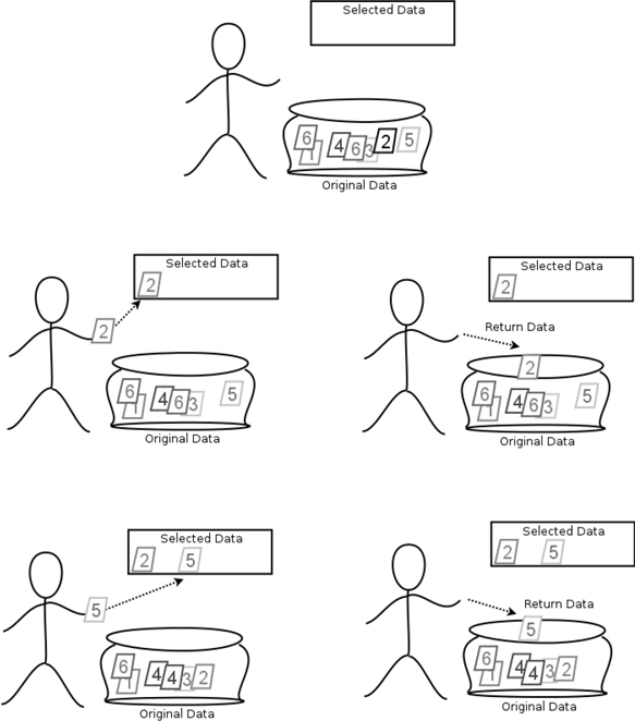
Figure 12.3 When we sample with replacement, examples are selected, recorded, and then returned to the cauldron.
So, how do we use bootstrapping to compute a bootstrap statistic? We randomly sample our source dataset, with replacement, until we generate a new bootstrap sample with the same number of elements as our original. We compute our statistic of interest on that bootstrap sample. We do that several times and then take the mean of those individual bootstrap sample statistics. Figure 12.4 shows the process visually for calculating the bootstrap mean.

Figure 12.4 We repeatedly calculate the value of the mean on bootstrap samples. We combine those values by taking their mean.
Let’s illustrate that idea with some code. We’ll start with the classic, nonbootstrap formula for the mean.
In [3]:
dataset = np.array([1,5,10,10,17,20,35])
def compute_mean(data):
    return np.sum(data) / data.size
compute_mean(dataset)
Out[3]:
14.0
Nothing too difficult there. One quick note: we could apply that calculation to the entire dataset and get the usual answer to the question, “What is the mean?” We could also apply compute_mean to other, tweaked forms of that dataset. We’ll get different answers to different questions.
Now, let’s pivot to the bootstrap technique. We’ll define a helper function to take a bootstrap sample—remember, it happens with replacement—and return it.
In [4]:
def bootstrap_sample(data):
    N   = len(data)
    idx = np.arange(N)
    bs_idx = np.random.choice(idx, N,
                              replace=True) # default added for clarity
    return data[bs_idx]
Now we can see what several rounds of bootstrap sampling and the means for those samples look like:
In [5]:
bsms = []
for i in range(5):
    bs_sample = bootstrap_sample(dataset)
    bs_mean = compute_mean(bs_sample)
    bsms.append(bs_mean)

    print(bs_sample, "{:5.2f}".format(bs_mean))
[35 10  1  1 10 10 10] 11.00
[20 35 20 20 20 20 20] 22.14
[17 10 20 10 10  5 17] 12.71
[20  1 10 35  1 17 10] 13.43
[17 10 10 10  1  1 10]  8.43
From those bootstrap sample means we can compute a single value—the mean of the means:
In [6]:
print("{:5.2f}".format(sum(bsms) / len(bsms)))
13.54
Here is the bootstrap calculation rolled up into a single function:
In [7]:
def compute_bootstrap_statistic(data, num_boots, statistic):
    ' repeatedly calculate statistic on num_boots bootstrap samples'
    # no comments from the peanut gallery
    bs_stats = [statistic(bootstrap_sample(data)) for i in range(num_boots)]
    # return the average of the calculated statistics
    return np.sum(bs_stats) / num_boots

bs_mean = compute_bootstrap_statistic(dataset, 100, compute_mean)
print("{:5.2f}".format(bs_mean))
13.86
The really interesting part is that we can compute just about any statistic using this same process. We’ll follow up on that idea now.
12.3.2 From Bootstrapping to Bagging
When we create a bagged learner, we are constructing a much more convoluted statistic: a learner in the form of a trained model. In what sense is a learner a statistic? Broadly, a statistic is any function of a group of data. The mean, median, min, and max are all calculations that we apply to a dataset to get a result. They are all statistics. Creating, fitting, and applying a learner to a new example—while a bit more complicated—is just calculating a result from a dataset.
I’ll prove it by doing it.
In [8]:
def make_knn_statistic(new_example):
    def knn_statistic(dataset):
        ftrs, tgt = dataset[:,:-1], dataset[:,-1]
        knn = neighbors.KNeighborsRegressor(n_neighbors=3).fit(ftrs, tgt)
        return knn.predict(new_example)
    return knn_statistic
The one oddity here is that we used a closure—we discussed these in Section 11.1. Here, our statistic is calculated with respect to one specific new example. We need to hold that test example fixed, so we can get down to a single value. Having done that trick, we have a calculation on the dataset—the inner function, knn_statistic—that we can use in the exact same way that we used compute_mean.
In [9]:
# have to slightly massage data for this scenario
# we use last example as our fixed test example
diabetes_dataset = np.c_[diabetes_ftrs, diabetes_tgt]

ks = make_knn_statistic(diabetes_ftrs[-1].reshape(1,-1))
compute_bootstrap_statistic(diabetes_dataset, 100, ks)
Out[9]:
74.00666666666667
Just like computing the mean will give us different answers depending on the exact dataset we use, the returned value from knn_statistic will depend on the data we pass into it.
We can mimic that process and turn it into our basic algorithm for bagging:
Sample the data with replacement.
Create a model and train it on that data.
Repeat.
To predict, we feed an example into each of the trained models and combine their predictions. The process, using decision trees as the component models, is shown in Figure 12.5.

Figure 12.5 As with the bootstrapped mean, we sample the dataset and generate a decision tree from each subdataset. Every tree has a say in the final prediction.
Here’s some pseudocode for a classification bagging system:
In [10]:
def bagged_learner(dataset, base_model, num_models=10):
    # pseudo-code: needs tweaks to run
    models = []
    for n in num_models:
        bs_sample = np.random.choice(dataset, N, replace=True)
        models.append(base_model().fit(*bs_sample))
    return models

def bagged_predict_class(models, example):
    # take the most frequent (mode) predicted class as result
    preds = [m.predict(example) for m in models]
    return pd.Series(preds).mode()
We can talk about some practical concerns of bagging using the bias-variance terminology we introduced in Section 5.6. (And you thought that was all just theoretical hand-waving!) Our process of combining many predictions is good at balancing out high variance: conceptually, we’re OK with overfitting in our base model. We’ll overfit and then let the averaging—or, here, taking the biggest vote getter with the mode—smooth out the rough edges. Bagging doesn’t help with bias, but it can help significantly reduce variance. In practice, we want the base_model to have a low bias.
Conceptually, since our learners are created from samples that are taken with replacement, the learners are independent of one another. If we really wanted to, we could train each of the different base models on a separate computer and then combine them together at the end. We could use this separation to great effect if we want to use parallel computing to speed up the training process.
12.3.3 Through the Random Forest
Random forests (RFs) are a specific type of a bagged learner built on top of decision trees. RFs use a variation on the decision trees we’ve seen. Standard decision trees take the best-evaluated feature of all the features to create a decision node. In contrast, RFs subselect a random set of features and then take the best of that subset. The goal is to force the trees to be different from each other. You can imagine that even over a random selection of the examples, a single feature might be tightly related to the target. This alpha feature would then be pretty likely to be chosen as the top split point in each tree. Let’s knock down the monarch of the hill.
Instead of a single feature being the top decision point in many bootstrapped trees, we’ll selectively ignore some features and introduce some randomness to shake things up. The randomness forces different trees to consider a variety of features. The original random forest algorithm relied on the same sort of majority voting that we described for bagging. However, sklearn’s version of RFs extracts class probabilities from each tree in the forest and then averages those to get a final answer: the class with the highest average probability is the winner.
If we start with our bagged_learner code from above, we still need to modify our tree-creation code—the component-model building step—from Section 8.2. It is a pretty simply modification which I’ve placed in italics:
Randomly select a subset of features for this tree to consider.
Evaluate the selected features and splits and pick the best feature-and-split.
Add a node to the tree that represents the feature-split.
For each descendant, work with the matching data and either:
If the targets are similar enough, return a predicted target.
If not, return to step 1 and repeat.
Using that pseudocode as our base estimator, together with the bagged_learner code, gets us a quick prototype of a random forest learning system.
Extreme Random Forests and Feature Splits One other variant—yet another bagged-tree (YABT)—is called an extreme random forest. No, this is not the X-Games of decision-tree sports. Here, extreme refers to adding yet another degree of randomness to the model creation process. Give a computer scientist an idea—replacing a deterministic method with randomness—and they will apply it everywhere. In extreme random forests, we make the following change to the component-tree building process:
Select split points at random and take the best of those.
So, in addition to randomly choosing what features are involved, we also determine what values are important by coin flipping. It’s amazing that this technique works—and it can work well indeed. Until now, I have not gone into great detail about the split selection process. I don’t really care to, since there are many, many discussions of it around. I particularly like how Foster and Provost approach it in their book that I reference at the end of the chapter.
Let me give you the idea behind making good split points with an example. Suppose we wanted to predict good basketball players from simple biometric data. Unfortunately for folks like myself, height is a really good predictor of basketball success. So, we might start by considering how height is related to a dataset of successful and—like myself—nonsuccessful basketball players. If we order all of the heights, we might find that people from 4’5” to 6’11” have tried to play basketball. If I introduce a split-point at 5’0”, I’ll probably have lots of unsuccessful players on the less-than side. That’s a relatively similar group of people when grouped by basketball success. But, on the greater-than side, I’ll probably have a real mix of both classes. We say that we have low purity above the split point and high purity below the split point. Likewise, if I set a split point at 6’5”, there are probably a lot of successful people on the high side, but the low side is quite mixed. Our goal is to find that just right split point on height that gives me as much information about the success measure—for both the taller and shorter folks—as possible. Segmenting off big heights and low heights gets me a lot of information. In the middle, other factors, such as the amount of time playing basketball, matter a lot.
So, extreme random forests don’t consider all possible split points. They merely choose a random subset of points to consider, evaluate those points, and take the best—of that limited set.
12.4 Boosting
I remember studying for vocabulary and geography tests using flash cards. I don’t know if the App Generation knows about these things. They were little pieces of paper—two-sided, like most pieces of paper—and on one side you would put a word or a noun or a concept and on the other side you would put a definition or an important characteristic of that thing. For example, one side might be gatto and the other side cat (for an Italian vocab test), or Lima on one side and capital of Peru on the other (for a world geography test).
Studying was a simple act of flipping through the flash cards—seeing one side and recalling the other. You could use both sides to go (1) from concept to definition or (2) from definition to concept. Now, typically, I wouldn’t keep all the cards in the deck. Some of the definitions and concepts became easy for me and I’d put those cards aside (Figure 12.6) so I could focus on the difficult concepts. Eventually, I whittled the deck down to a fairly small pile—the hard stuff—which I kept studying until the exam.

Figure 12.6 When studying with flashcards, we can selectively remove the easy cards and focus our attention on the hard examples. Boosting uses a similar approach.
The process of taking cards out of the deck is a bit like weighting the likelihood of seeing those cards but in an extreme way: it takes the probability down to zero. Now, if I really wanted to be thorough, instead of removing the easy cards, I could add duplicates of the hard cards. The effect would be similar: hard cards would be seen more often and easy cards would be seen less. The difference is that the process would be gradual.
We can apply this same idea—focusing on the hard examples—to a learning system. We start by fitting a Simple-McSimple Model to some hard data. Not surprisingly, we get a lot of examples wrong. But surprisingly, we do get a few right. We refocus our efforts on the harder examples and try again. That repeated process of focusing our efforts on harder examples—and considering the easier examples done(-ish)—is the heart of boosting.
12.4.1 Boosting Details
With boosting, we learn a simple model. Then, instead of resampling equally from the base dataset, we focus on the examples that we got wrong and develop another model. We repeat that process until we are satisfied or run out of time. Thus, boosting is a sequential method and the learners developed at later stages depend on what happened at earlier stages. While boosting can be applied to any learning model as the primitive component model, often we use decision stumps—decision trees with only one split point. Decision stumps have a depth of one.
We haven’t talked about what learning with weighted data means. You can think of it in two different ways. First, if we want to perform weighted training and example A has twice the weight of example B, we’ll simply duplicate example A twice in our training set and call it a day. The alternative is to incorporate the weighting in our error or loss measures. We can weight errors by the example weight and get a weighted error. Then, we find the best knob settings with respect to the weighted errors, not raw errors.
In a very raw, pseudocode form, these steps look like:
Initialize example weights to and m to zero.
Repeat until done:
Increment m.
Fit a new classifier (often a stump), Cm, to the weighted data.
Compute weighted error of new classifier.
The classifier weight, wgtm, is function of weighted errors.
Update example weights based on old example weights, classifier errors, and classifier weights.
For new example and m repeats, output a prediction from the majority vote of C weighted by wgt.
We can take some massive liberties (don’t try this at home!) and write some Pythonic pseudocode:
In [11]:
def my_boosted_classifier(base_classifier, bc_args,
                          examples, targets, M):
    N = len(examples)
    data_weights = np.full(N, 1/N)
    models, model_weights = [], []

    for i in range(M):
        weighted_dataset = reweight((examples,targets),
                                    data_weights)
        this_model = base_classifier(*bc_args).fit(*weighted_dataset)

        errors = this_model.predict(examples) != targets
        weighted_error = np.dot(weights, errors)

        # magic reweighting steps
        this_model_wgt = np.log(1-weighted_error)/weighted_error
        data_weights   *= np.exp(this_model_wgt * errors)
        data_weights   /= data_weights.sum() # normalize to 1.0

        models.append(this_model)
        model_weights.append(this_model_wgt)

    return ensemble.VotingClassifier(models,
                                     voting='soft',
                                     weights=model_weights)
You’ll notice a few things here. We picked a value of M out of a hat. Certainly, that gives us a deterministic stopping point: we’ll only do M iterations. But we could introduce a bit more flexibility here. For example, sklearn stops its discrete AdaBoost—a specific boosting variant, similar to what we used here—when either the accuracy hits 100% or this_model starts doing worse than a coin flip. Also, instead of reweighting examples, we could perform weighted bootstrap sampling—it’s simply a different way to prioritize some data over another.
Boosting very naturally deals with bias in our learning systems. By combining many simple, highly biased learners, boosting reduces the overall bias in the results. Boosting can also reduce variance.
In boosting, unlike bagging, we can’t build the primitive models in parallel. We need to wait on the results of one pass so we can reweight our data and focus on the hard examples before we start our next pass.
12.4.1.1 Improvements with Boosting Iterations
The two major boosting classifiers in sklearn are GradientBoostingClassifier and AdaBoostClassifier. Each can be told the maximum number of component estimators—our M argument to my_boosted_classifier—to use through n_estimators. I’ll leave details of the boosters to the end notes, but here are a few tidbits. AdaBoost is the classic forebearer of modern boosting algorithms. Gradient Boosting is a new twist that allows us to plug in different loss functions and get different models as a result. For example, if we set loss="exponential" with the GradientBoostingClassifier, we get a model that is basically AdaBoost. The result gives us code similar to my_boosted_classifier.
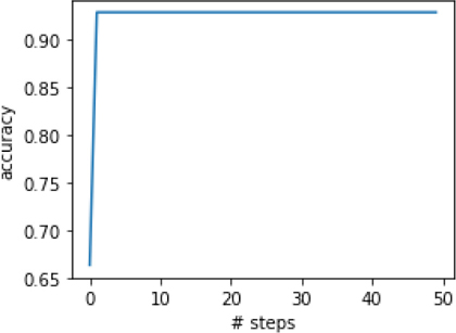
Since boosting is an iterative process, we can reasonably ask how our model improves over the cycles of reweighting. sklearn makes it relatively easy to access that progress through staged_predict. staged_predict operates like predict except it follows the predictions made on examples at each step—or stage—of the learning process. We need to convert those predictions into evaluation metrics if we want to quantify the progress.
In [12]:
model = ensemble.AdaBoostClassifier()
stage_preds = (model.fit(iris_train_ftrs, iris_train_tgt)
                    .staged_predict(iris_test_ftrs))
stage_scores = [metrics.accuracy_score(iris_test_tgt,
                                       pred) for pred in stage_preds]
fig, ax = plt.subplots(1,1,figsize=(4,3))
ax.plot(stage_scores)
ax.set_xlabel('# steps')
ax.set_ylabel('accuracy');
12.5 Comparing the Tree-Ensemble Methods
Let’s now compare how these team-based methods work on the digits data. We’ll start with two simple baselines: a single decision stump (equivalent to a max_depth=1 tree) and a single max_depth=3 tree. We’ll also build 100 different forests with a number of tree stumps going from 1 to 100.
In [13]:
def fit_predict_score(model, ds):
    return skms.cross_val_score(model, *ds, cv=10).mean()

stump  = tree.DecisionTreeClassifier(max_depth=1)
dtree  = tree.DecisionTreeClassifier(max_depth=3)
forest = ensemble.RandomForestClassifier(max_features=1, max_depth=1)
tree_classifiers = {'stump' : stump, 'dtree' : dtree, 'forest': forest}

max_est = 100
data = (digits_ftrs, digits_tgt)
stump_score   = fit_predict_score(stump, data)
tree_score    = fit_predict_score(dtree, data)
forest_scores = [fit_predict_score(forest.set_params(n_estimators=n),
                                   data)
                 for n in range(1,max_est+1)]
We can view those results graphically:
In [14]:
fig, ax = plt.subplots(figsize=(4,3))

xs = list(range(1,max_est+1))
ax.plot(xs, np.repeat(stump_score, max_est), label='stump')
ax.plot(xs, np.repeat(tree_score, max_est),  label='tree')
ax.plot(xs, forest_scores, label='forest')

ax.set_xlabel('Number of Trees in Forest')
ax.set_ylabel('Accuracy')
ax.legend(loc='lower right');

Comparing the forests to the two baselines shows that a single-stump forest acts a lot like—unsurprisingly—a stump. But then, as the number of stumps grows, we quickly outperform even our moderately sized tree.
Now, to see how the boosting methods progress over time and to make use of cross-validation—to make sure we’re comparing apples to apples—we need to manually manage a bit of the cross-validation process. It’s not complicated, but it is slightly ugly. Essentially, we need to generate the fold indices by hand with StratifiedKFold (we looked at this in Section 5.5.2) and then use those indices to select the proper parts of our dataset. We could simply place this code inline, below, but that really obscures what we’re trying to do.
In [15]:
def my_manual_cv(dataset, k=10):
    ' manually generate cv-folds from dataset '
    # expect ftrs, tgt tuple
    ds_ftrs, ds_tgt = dataset
    manual_cv = skms.StratifiedKFold(k).split(ds_ftrs,
                                              ds_tgt)
    for (train_idx, test_idx) in manual_cv:
        train_ftrs = ds_ftrs[train_idx]
        test_ftrs  = ds_ftrs[test_idx]
        train_tgt  = ds_tgt[train_idx]
        test_tgt   = ds_tgt[test_idx]

        yield (train_ftrs, test_ftrs,
               train_tgt, test_tgt)
For this comparison, we’ll use a deviance loss for our gradient boosting classifier. The result is that our classifier acts like logistic regression. We tinker with one important parameter to give AdaBoostClassifier a legitimate shot at success on the digits data. We adjust the learning_rate which is an additional factor—literally, a multiplier—on the weights of the estimators. You can think of it as multiplying this_model_weight in my_boosted_classifier.
In [16]:
AdaBC  = ensemble.AdaBoostClassifier
GradBC = ensemble.GradientBoostingClassifier
boosted_classifiers = {'boost(Ada)' : AdaBC(learning_rate=2.0),
                       'boost(Grad)' : GradBC(loss="deviance")}
mean_accs = {}
for name, model in boosted_classifiers.items():
    model.set_params(n_estimators=max_est)
    accs = []
    for tts in my_manual_cv((digits_ftrs, digits_tgt)):
        train_f, test_f, train_t, test_t = tts
        s_preds = (model.fit(train_f, train_t)
                        .staged_predict(test_f))
        s_scores = [metrics.accuracy_score(test_t, p) for p in s_preds]
        accs.append(s_scores)
    mean_accs[name] = np.array(accs).mean(axis=0)
mean_acc_df = pd.DataFrame.from_dict(mean_accs,orient='columns')
Pulling out the individual, stage-wise accuracies is a bit annoying. But the end result is that we can compare the number of models we are combining between the different ensembles.
In [17]:
xs = list(range(1,max_est+1))
fig, (ax1, ax2) = plt.subplots(1,2,figsize=(8,3),sharey=True)
ax1.plot(xs, np.repeat(stump_score, max_est), label='stump')
ax1.plot(xs, np.repeat(tree_score, max_est),  label='tree')
ax1.plot(xs, forest_scores, label='forest')
ax1.set_ylabel('Accuracy')
ax1.set_xlabel('Number of Trees in Forest')
ax1.legend()

mean_acc_df.plot(ax=ax2)
ax2.set_ylim(0.0, 1.1)
ax2.set_xlabel('# Iterations')
ax2.legend(ncol=2);

After adding more trees to the forest and letting more iterations pass for AdaBoost, the forest and AdaBoost have broadly similar performance (near 80% accuracy). However, the AdaBoost classifier doesn’t seem to perform nearly as well as the GradientBoosting classifier. You can play around with some hyperparameters—GridSearch is seeming mighty useful about now—to see if you can improve any or all of these.
12.6 EOC
12.6.1 Summary
The techniques we’ve explored in this chapter bring us to some of the more powerful models available to the modern machine learning practitioner. They build conceptually and literally on top of the models we’ve seen throughout our tour of learning methods. Ensembles bring together the best aspects of teamwork to improve learning performance compared to individuals.
12.6.2 Notes
In machine learning, the specialist learning scenario typically has terms like additive, mixture, or expert in the name. The key is that the component models only apply to certain areas of the input. We can extend this to a fuzzy specialist scenario where applying to a region need not be a binary yes or no but can be given by a weight. Models can gradually turn on and off in different regions.
Not to get too meta on you, but many simple learners—linear regression and decision trees, I’m looking at you—can be viewed as ensembles of very simple learning components combined together. For example, we combine multiple decision stumps to create a standard decision tree. To make a prediction, a decision tree asks questions of its decision stumps and ends up with an answer. Likewise, a linear regression takes the contribution of each feature and then adds up—combines with a dot product, to be specific—those single-feature predictions into a final answer. Now, we don’t normally talk about decision trees and linear regression as ensembles. Just keep in mind that there is nothing magical about taking simple answers or predictions and combining them in some interesting and useful ways.
We computed a number of bootstrap estimates of a statistic: first the mean and then classifier predictions. We can use the same technique to compute a bootstrap estimate of variability (variance)—using the usual formula for variance—and we can perform other statistical analyses in a similar manner. These methods are very broadly applicable in scenarios that don’t lend themselves to simple formulaic calculations. However, they do depend on some relatively weak but extremely technical assumptions—compact differentiability is the term to google—to have theoretical support. Often, we charge bravely ahead, even without complete theoretical support.
Boosting Boosting is really amazing. It can continue to improve its testing performance even after its training performance is perfect. You can think about this as smoothing out unneeded wiggles as it continues iterating. While it is fairly well agreed that bagging reduces variance and boosting reduces bias, it is less well agreed that boosting reduces variance. My claim to this end is based on technical report by Breiman, “Bias, Variance, and Arcing Classifiers.” Here, arcing is a close cousin to boosting. An additional useful point from that report: bagging is most useful for unstable—high-variance—methods like decision trees.
The form of boosting we discussed is called AdaBoost—for adaptive boosting. The original form of boosting—pre-AdaBoost—was quite theoretical and had issues that rendered it impractical in many scenarios. AdaBoost resolved those issues, and subsequent research connected AdaBoost to fitting models with an exponential loss. In turn, substituting other loss functions led to boosting methods appropriate for different kinds of data. In particular, gradient boosting lets us swap out a different loss function and get different boosted learners, such as boosted logistic regression. My boosting pseudocode is based on Russell and Norvig’s excellent Artificial Intelligence: A Modern Approach.
Aside from sklearn, there are other boosting implementations out there. xgboost—for extreme gradient boosting—is the newest kid on the block. It uses a technique—an optimization strategy—that produces better weights as it calculates the weights of the component models. It also uses slightly less tiny component models. Coupling better weighting with more complex component models, xgboost has a cult-like following on Kaggle (a social website, with competitions, for machine learning enthusiasts).
We can’t always use xgboost’s technique but we can use it in common learning scenarios. Here’s a super quick code demo:
In [18]:
# conda install py-xgboost
import xgboost
# gives us xgboost.XGBRegressor, xgboost.XGBClassifier
# which interface nicely with sklearn
# see docs at
# http://xgboost.readthedocs.io/en/latest/parameter.html
xgbooster = xgboost.XGBClassifier(objective="multi:softmax")
scores = skms.cross_val_score(xgbooster, iris.data, iris.target, cv=10)
print(scores)
[1. 0.9333 1. 0.9333 0.9333 0.9333 0.9333 0.9333 1. 1. ]
12.6.3 Exercises
Ensemble methods are very, very powerful—but they come at a computational cost. Evaluate and compare the resource usage (memory and time) of several different tree-based learners: stumps, decision trees, boosted stumps, and random forests.
Create a voting classifier with a few—five—relatively old-school base learners, for example linear regression. You can feed the base learners with datasets produced by cross-validation, if you’re clever. (If not, you can MacGyver something together—but that just means being clever in a different way!) Compare the bias and variance—underfitting and overfitting—of the base method developed on the whole training set and the voting method by assessing them on training and testing sets and overlaying the results. Now, repeat the same process using bagged learners. If you are using something besides decision trees, you might want to look at
sklearn.ensemble.BaggingRegressor.You can implement a bagged classifier by using some of the code we wrote along with
sklearn’sVotingClassifier. It gives you a choice in how you use the votes: they can behard(everyone gets one vote and majority wins) orsoft(everyone gives a probability weight to a class and we add those up—the biggest value wins).sklearn’s random forest uses the equivalent ofsoft. You can compare that with ahardvoting mechanism.softis recommended when the probabilities of the base models are well calibrated, meaning they reflect the actual probability of the event occurring. We aren’t going to get into it, but some models are not well calibrated. They can classify well, but they can’t give reasonable probabilities. You can think of it as finding a good boundary, but not having insight into what goes on around the boundary. Assessing this would require knowing real-world probabilities and comparing them to the probabilities generated by the model—that’s a step beyond simply having target classes.Since we like to use boosting with very simple models, if we turn our attention to linear regression we might think about using simple constant models as our base models. That is just a horizontal line: y = b. Compare good old-fashioned linear regression with boosted constant regressions on a regression dataset.
What happens if we use deeper trees in ensembles? For example, what happens if you use trees of depth two or three as the base learners in boosting? Do you see any significant improvements or failures?
We saw
AdaBoostlose out toGradientBoosting. Use aGridSearchto try several different parameter values for each of these ensemble methods and compare the results. In particular, you might try to find a good value for the learning rate.