
15. Connections, Extensions, and Further Directions
In [1]:
from mlwpy import *
15.1 Optimization
When we try to find a best line, curve, or tree to match our data—which is our main goal in training—we want to have an automated method do the work for us. We’re not asking the hot dog vendor for a quick stock tip: we need an algorithm. One of the principal—principled—ways to do this is by assessing our cost and looking for ways to lower that cost. Remember, the cost is a combination of the loss—how well our model’s predictions match the training data—and the complexity of the model. When we minimize cost, we try to achieve a small loss while keeping a low complexity. We can’t always get to that ideal, but that’s our goal.
When we train a learning model, one of the easiest parameters to think about is the weights—from linear or logistic regression—that we combine with the feature values to get our predictions. Since we get to adjust the weights, we can look at the effect of adjusting them and see what happens to the cost. If we have a definition of the cost—a cost function, perhaps drawn as a graph—we can turn the adjusting process into a question. From where we are—that is, from our current weights and the cost we get by using them—what small adjustments to the weights can we make? Is there a direction that we can go that will result in a lower cost? A way to think about this visually is to ask what direction is downhill on our cost function. Let’s look at an example.
In [2]:
xs = np.linspace(-5,5)
ys = xs**2

fig, ax = plt.subplots(figsize=(4,3))
ax.plot(xs, ys)

# better Python:
# pt = co.namedtuple('Point', ['x', 'y'])(3,3**2)
pt_x, pt_y = 3, 3**2
ax.plot(pt_x, pt_y, 'ro')

line_xs = pt_x + np.array([-2, 2])
# line ys = mid_point + (x amount) * slope_of_line
# one step right gets one "slope of line" increase in that line's up
line_ys = 3**2 + (line_xs - pt_x) * (2 * pt_x)
ax.plot(line_xs, line_ys, 'r-')
ax.set_xlabel('weight')
ax.set_ylabel('cost');

In this simple example, if we put an imaginary ball at the red dot, it would roll downward to the left. The red line represents the slope—how steep the blue graph is—at that point. You can imagine that if we are trying to find a low point, we want to follow the slope—with Jack and Jill down the proverbial hill. You might also find it reasonable to be more confident in our direction if the slope is steeper—that is, we can roll down the hill faster if there is a steeper slope. If we do that, here’s one take on what can happen.
From the starting point of weight = 3 that we just saw, we can take a step down the hill by moving to the left. We’ll take a step that is moderated by the slope at our current point. Then we’ll repeat the process. We’ll try this ten times and see what happens. Note that we could have picked the starting point randomly—we’d have to be pretty lucky for it to be the minimum.
In [3]:
weights = np.linspace(-5,5)
costs   = weights**2
fig, ax = plt.subplots(figsize=(4,3))
ax.plot(weights, costs, 'b')

# current best guess at the minimum
weight_min = 3

# we can follow the path downhill from our starting point
# and find out the weight value where our initial, blue graph is
# (approximately) the lowest
for i in range(10):
    # for a weight, we can figure out the cost
    cost_at_min = weight_min**2
    ax.plot(weight_min, cost_at_min, 'ro')

    # also, we can figure out the slope (steepness)
    # (via a magic incantation called a "derivative")
    slope_at_min = 2*weight_min

    # new best guess made by walking downhill
    step_size = .25
    weight_min = weight_min - step_size * slope_at_min

ax.set_xlabel('weight value')
ax.set_ylabel('cost')
print("Approximate location of blue graph minimum:", weight_min)
Approximate location of blue graph minimum: 0.0029296875

We gradually approach weight = 0 which is the actual minimum of the blue curve defined by weight2. In this example, we never really went past the low point because we took relatively small steps (based on the step_size = .25 in the weight_min assignment). You can imagine that if we took slightly bigger steps, we might shoot beyond the low point. That’s OK. We would then recognize that the downhill direction is now to the right and we can follow that path down. There are many details I’m sweeping under the carpet—but we can eventually settle in on the low point. In reality, we might only get a value very close to zero—0.0000000001, perhaps—but that is probably good enough.
We can apply many different strategies to find the minimum. We don’t have to do the downhill walking by hand—or even code it by hand. The general basket of techniques to do this is called mathematical optimization. We’ll make use of one optimizer that is built into scipy, called fmin. Since that is a really boring name, we’ll call it the magical_minimum_finder.
In [4]:
from scipy.optimize import fmin as magical_minimum_finder
def f(x):
    return x**2

magical_minimum_finder(f, [3], disp=False)
Out[4]:
array([-0.])
From a starting point of 3, magical_minimum_finder was able to locate the input value to f that resulted in the lowest output value. That result is analogous to what we want if we have weights as the inputs and a cost as the output. We now have one tool to use for finding minimum costs.
15.2 Linear Regression from Raw Materials
Now that we have a tool to minimize functions, can we build a linear regression system using that tool? Let’s step back out to a 40,000-foot view of learning. When we try to learn something, we are trying to fit the parameters of a model to some training data. In linear regression, our parameters are weights (m, b or wi) that we manipulate to make the features match the target. That’s also a quick review of our most important vocabulary.
Let’s get started by creating some simple synthetic data. To simplify a few things—and maybe complicate others—I’m going to pull a +1 trick. I’m going to do that by adding a column of ones to data as opposed to putting the +1 in the model.
In [5]:
linreg_ftrs_p1 = np.c_[np.arange(10), np.ones(10)] # +1 trick in data

true_wgts  = m,b = w_1, w_0 = 3,2
linreg_tgt = rdot(true_wgts, linreg_ftrs_p1)

linreg_table = pd.DataFrame(linreg_ftrs_p1,
                            columns=['ftr_1', 'ones'])
linreg_table['tgt'] = linreg_tgt
linreg_table[:3]
Out[5]:
|
ftr_1 |
ones |
tgt |
|---|---|---|---|
0 |
0.0000 |
1.0000 |
2.0000 |
1 |
1.0000 |
1.0000 |
5.0000 |
2 |
2.0000 |
1.0000 |
8.0000 |
We’ve made a super simple dataset that only has one interesting feature. Still, it’s complicated enough that we can’t get the answer—the right weights for a fit model—for free. Well, we could by peeking at the code we used to create the data, but we won’t do that. Instead, to find good weights, we’ll pull out magical_minimum_finder to do the heavy lifting for us. To use magical_minimum_finder, we have to define the loss that we get from our predictions versus the real state of the world in the target. We’ll do this in several steps. We have to explicitly define our learning model and the loss. We’ll also define an ultra simple weight penalty—none, no penalty—so we can make a full-fledged cost.
In [6]:
def linreg_model(weights, ftrs):
    return rdot(weights, ftrs)

def linreg_loss(predicted, actual):
    errors = predicted - actual
    return np.dot(errors, errors) # sum-of-squares

def no_penalty(weights):
    return 0.0
Now, you may have noticed that when we used magical_minimum_finder, we had to pass a Python function that took one—and only one—argument and did all of its wonderful minimizing work. From that single argument, we have to somehow convince our function to make all the wonderful fit, loss, cost, weight, and train components of a learning method. That seems difficult. To make this happen, we’ll use a Python trick: we will write one function that produces another function as its result. We did this in Section 11.2 when we created an adding function that added a specific value to an input value. Here, we’ll use the same technique to wrap up the model, loss, penalty, and data components as a single function of the model parameters. Those parameters are the weights we want to find.
In [7]:
def make_cost(ftrs, tgt,
              model_func, loss_func,
              c_tradeoff, complexity_penalty):
    ' build an optimization problem from data, model, loss, penalty '
    def cost(weights):
        return (loss_func(model_func(weights, ftrs), tgt) +
                c_tradeoff * complexity_penalty(weights))
    return cost
I’ll be honest. That’s a bit tricky to interpret. You can either (1) trust me that make_cost plus some inputs will set up a linear regression problem on our synthetic data or (2) spend enough time reading it to convince yourself that I’m not misleading you. If you want the fast alternative, go for (1). If you want the rock star answer, go for (2). I suppose I should have mentioned alternative (3) where you would simply say, “I have no clue. Can you show me that it works?” Good call. Let’s see what happens when we try to use make_cost to build our cost function and then minimize it with magical_minimum_finder.
In [8]:
# build linear regression optimization problem
linreg_cost = make_cost(linreg_ftrs_p1, linreg_tgt,
                        linreg_model, linreg_loss,
                        0.0, no_penalty)
learned_wgts = magical_minimum_finder(linreg_cost, [5,5], disp=False)

print("   true weights:", true_wgts)
print("learned weights:", learned_wgts)
   true weights: (3, 2)
learned weights: [3. 2.]
Well, that should be a load off of someone’s shoulders. Building that cost and magically finding the least cost weights led to—wait for it—exactly the true weights that we started with. I hope you are suitably impressed. Now, we didn’t make use of a penalty. If you recall from Chapter 9, we moved from a cost based on predicted targets to a loss based on those predictions plus a penalty for complex models. We did that to help prevent overfitting. We can add complexity penalties to our make_cost process by defining something more interesting than our no_penalty. The two main penalties we discussed in Section 9.1 were based on the absolute value and the squares of the weights. We called these L1 and L2 and we used them to make the lasso and ridge regression methods. We can build cost functions that effectively give us lasso and ridge regression. Here are the penalties we need:
In [9]:
def L1_penalty(weights):
    return np.abs(weights).sum()

def L2_penalty(weights):
    return np.dot(weights, weights)
And we can use those to make different cost functions:
In [10]:
# linear regression with L1 regularization (lasso regression)
linreg_L1_pen_cost = make_cost(linreg_ftrs_p1, linreg_tgt,
                               linreg_model, linreg_loss,
                               1.0, L1_penalty)
learned_wgts = magical_minimum_finder(linreg_L1_pen_cost, [5,5], disp=False)

print("   true weights:", true_wgts)
print("learned weights:", learned_wgts)
   true weights: (3, 2)
learned weights: [3.0212 1.8545]
You’ll notice that we didn’t get the exact correct weights this time. Deep breath—that’s OK. Our training data had no noise in it. As a result, the penalties on the weights actually hurt us.
We can follow the same template to make ridge regression:
In [11]:
# linear regression with L2 regularization (ridge regression)
linreg_L2_pen_cost = make_cost(linreg_ftrs_p1, linreg_tgt,
                               linreg_model, linreg_loss,
                               1.0, L2_penalty)
learned_wgts = magical_minimum_finder(linreg_L2_pen_cost, [5,5], disp=False)

print("   true weights:", true_wgts)
print("learned weights:", learned_wgts)
   true weights: (3, 2)
learned weights: [3.0508 1.6102]
Again, we had perfect data so penalties don’t do us any favors.
15.2.1 A Graphical View of Linear Regression
We can represent the computations we just performed as a flow of data through a graph. Figure 15.1 shows all the pieces in a visual form.

Figure 15.1 A graphical view of linear regression.
15.3 Building Logistic Regression from Raw Materials
So, we were able to build a simple linear regression model using some Python coding tricks and magical_minimum_finder. That’s pretty cool. Let’s make it awesome by showing how we can do classification—logistic regression—using the same steps: define a model and a cost. Then we minimize the cost. Done.
Again, we’ll get started by generating some synthetic data. The generation process is a hint more complicated. You might remember that the linear regression part of logistic regression was producing the log-odds. To get to an actual class, we have to convert the log-odds into probabilities. If we’re simply interested in the target classes, we can use those probabilities to pick classes. However, when we select a random value and compare it to a probability, we don’t get a guaranteed result. We have a probability of a result. It’s a random process that is inherently noisy. So, unlike the noiseless regression data we used above, we might see benefits from regularization.
In [12]:
logreg_ftr = np.random.uniform(5,15, size=(100,))

true_wgts  = m,b = -2, 20
line_of_logodds = m*logreg_ftr + b
prob_at_x  = np.exp(line_of_logodds) / (1 + np.exp(line_of_logodds))

logreg_tgt = np.random.binomial(1, prob_at_x, len(logreg_ftr))

logreg_ftrs_p1 = np.c_[logreg_ftr,
                       np.ones_like(logreg_ftr)]

logreg_table = pd.DataFrame(logreg_ftrs_p1,
                            columns=['ftr_1','ones'])
logreg_table['tgt'] = logreg_tgt
display(logreg_table.head())
|
ftr_1 |
ones |
tgt |
|---|---|---|---|
0 |
8.7454 |
1.0000 |
1 |
1 |
14.5071 |
1.0000 |
0 |
2 |
12.3199 |
1.0000 |
0 |
3 |
10.9866 |
1.0000 |
0 |
4 |
6.5602 |
1.0000 |
1 |
Graphically, the classes—and their probabilities—look like
In [13]:
fig, ax = plt.subplots(figsize=(6,4))
ax.plot(logreg_ftr, prob_at_x, 'r.')
ax.scatter(logreg_ftr, logreg_tgt, c=logreg_tgt);

So, we have two classes here, 0 and 1, represented by the yellow and purple dots. The yellow dots fall on the horizontal line at y = 1 and the purple dots fall on the horizontal line at y = 0. We start off with pure 1s. As our input feature gets bigger, the likelihood of class 1 falls off. We start seeing a mix of 1 and 0. Eventually, we see only 0s. The mix of outcomes is controlled by the probabilities given by the red dots on the curving path that falls from one to zero. On the far left, we are flipping a coin that has an almost 100% chance of coming up 1, and you’ll notice that we have lots of 1 outcomes. On the right-hand side, the red dots are all near zero—we have almost a zero percent chance of coming up with a 1. In the middle, we have moderate probabilities of coming up with ones and zeros. Between 9 and 11 we get some 1s and some 0s.
Creating synthetic data like this may give you a better idea of where and what the logistic regression log-odds, probabilities, and classes come from. More practically, this data is just hard enough to classify to make it interesting. Let’s see how we can classify it with our magical_minimum_finder.
15.3.1 Logistic Regression with Zero-One Coding
We’re not going to have much fuss creating our minimization problem. Our model—predicting the log-odds—is really the same as the linear regression model. The difference comes in how we assess our loss. The loss we’ll use has many different names: logistic loss, log-loss, or cross-entropy loss. Suffice it to say that it measures the agreement between the probabilities we see in the training data and our predictions. Here’s the loss for one prediction:
pactual is known, since we know the target class. ppred is unknown and can wave gradually from 0 to 1. If we put that loss together with target values of zero and one and shake it up with some algebra, we get another expression which I’ve translated into code logreg_loss_01.
In [14]:
# for logistic regression
def logreg_model(weights, ftrs):
    return rdot(weights, ftrs)

def logreg_loss_01(predicted, actual):
    # sum(-actual log(predicted) - (1-actual) log(1-predicted))
    # for 0/1 target works out to
    return np.sum(- predicted * actual + np.log(1+np.exp(predicted)))
So, we have our model and our loss. Does it work?
In [15]:
logreg_cost = make_cost(logreg_ftrs_p1, logreg_tgt,
                        logreg_model, logreg_loss_01,
                        0.0, no_penalty)
learned_wgts = magical_minimum_finder(logreg_cost, [5,5], disp=False)

print("   true weights:", true_wgts)
print("learned weights:", learned_wgts)
   true weights: (-2, 20)
learned weights: [-1.9774 19.8659]
Not too bad. Not as exact as we saw with good old-fashioned linear regression, but pretty close. Can you think of why? Here’s a hint: did we have noise in our classification examples? Put differently, were there some input values that could have gone either way in terms of their output class? Second hint: think about the middle part of the sigmoid.
Now, let’s see if regularization can help us:
In [16]:
# logistic regression with penalty
logreg_pen_cost = make_cost(logreg_ftrs_p1, logreg_tgt,
                            logreg_model, logreg_loss_01,
                            0.5, L1_penalty)
learned_wgts = magical_minimum_finder(logreg_pen_cost, [5,5], disp=False)
print("   true weights:", true_wgts)
print("learned weights:", learned_wgts)
   true weights: (-2, 20)
learned weights: [-1.2809 12.7875]
The weights are different and have gone the wrong way. However, I simply picked our tradeoff between prediction accuracy and complexity C out of a hat. We shouldn’t therefore read too much into this: it’s a very simple dataset, there aren’t too many data points, and we only tried one value of C. Can you find a better C?
15.3.2 Logistic Regression with Plus-One Minus-One Coding
Before we leave logistic regression, let’s add one last twist. Conceptually, there shouldn’t be any difference between having classes that are cat and dog, or donkey and elephant, or zero and one, or +one and –one. We just happened to use 0/1 above because it played well with the binomial data generator we used to flip coins. In reality, there are nice mathematical reasons behind that as well. We’ll ignore those for now.
Since the mathematics for some other learning models can be more convenient using –1/+1, let’s take a quick look at logistic regression with ±1. The only difference is that we need a slightly different loss function. Before we get to that, however, let’s make a helper to deal with converting 01 data to ±1 data.
In [17]:
def binary_to_pm1(b):
    ' map {0,1} or {False,True} to {-1, +1} '
    return (b*2)-1
binary_to_pm1(0), binary_to_pm1(1)
Out[17]:
(-1, 1)
Here, we’ll update the loss function to work with the ±1 data. Mathematically, we start with the same log loss expression we had above, work through some slightly different algebra using the ±1 values, and get the logreg_loss_pm1. The two logreg_loss functions are just slightly different code expressions of the same mathematical idea.
In [18]:
# for logistic regression
def logreg_model(weights, ftrs):
    return rdot(weights, ftrs)

def logreg_loss_pm1(predicted, actual):
    # -actual log(predicted) - (1-actual) log(1-predicted)
    # for +1/-1 targets, works out to:
    return np.sum(np.log(1+np.exp(-predicted*actual)))
With a model and a loss, we can perform our magical minimization to find good weights.
In [19]:
logreg_cost = make_cost(logreg_ftrs_p1, binary_to_pm1(logreg_tgt),
                        logreg_model, logreg_loss_pm1,
                        0.0, no_penalty)
learned_wgts = magical_minimum_finder(logreg_cost, [5,5], disp=False)

print("   true weights:", true_wgts)
print("learned weights:", learned_wgts)
   true weights: (-2, 20)
learned weights: [-1.9774 19.8659]
While the weights are nice, I’m curious about what sort of classification performance these weights give us. Let’s take a quick look. We need to convert the weights into actual classes. We’ll do that with another helper that knows how to convert weights into probabilities and then into classes.
In [20]:
def predict_with_logreg_weights_to_pm1(w_hat, x):
    prob = 1 / (1 + np.exp(rdot(w_hat, x)))
    thresh = prob < .5
    return binary_to_pm1(thresh)

preds = predict_with_logreg_weights_to_pm1(learned_wgts, logreg_ftrs_p1)
print(metrics.accuracy_score(preds, binary_to_pm1(logreg_tgt)))
0.93
Good enough. Even if the weights are not perfect, they might be useful for prediction.
15.3.3 A Graphical View of Logistic Regression
We can look at the logistic regression in the same graphical way we looked at the mathematics of the linear regression in Figure 15.1. The one piece that is a bit more complicated in the logistic regression is the form. You might remember that fraction as our logistic or sigmoid function. If we’re content with using the name “logistic” to represent that function, we can draw the mathematical relationships as in Figure 15.2.

Figure 15.2 A graphical view of logistic regression.
15.4 SVM from Raw Materials
We’ve been on this journey for quite a long time now. I can’t really pull any new tricks on you. You probably won’t be too surprised if I tell you that we can do the same process with other learning models. In particular, let’s see what SVM looks like when we build it from primitive components. Again, our only difference is that we’ll have a slightly different loss function.
In [21]:
# for SVC
def hinge_loss(predicted, actual):
    hinge = np.maximum(1-predicted*actual, 0.0)
    return np.sum(hinge)

def predict_with_svm_weights(w_hat, x):
    return np.sign(rdot(w_hat,x)).astype(np.int)
SVM plays most nicely with ±1 data. We won’t fight it. Since the SVM model is just the dot product, we won’t even bother giving it a special name.
In [22]:
svm_ftrs = logreg_ftrs_p1
svm_tgt  = binary_to_pm1(logreg_tgt)  # svm "demands" +/- 1

# svm model is "just" rdot, so we don't define it separately now
svc_cost = make_cost(svm_ftrs, svm_tgt, rdot,
                     hinge_loss, 0.0, no_penalty)
learned_weights = magical_minimum_finder(svc_cost, [5,5], disp=False)

preds = predict_with_svm_weights(learned_weights, svm_ftrs)
print('no penalty accuracy:',
      metrics.accuracy_score(preds, svm_tgt))
no penalty accuracy: 0.91
As we did with linear and logistic regression, we can add a penalty term to control the weights.
In [23]:
# svc with penalty
svc_pen_cost = make_cost(svm_ftrs, svm_tgt, rdot,
                         hinge_loss, 1.0, L1_penalty)
learned_weights = magical_minimum_finder(svc_pen_cost, [5,5], disp=False)

preds = predict_with_svm_weights(learned_weights, svm_ftrs)
print('accuracy with penalty:',
      metrics.accuracy_score(preds, svm_tgt))
accuracy with penalty: 0.91
Now would be a great time to give you a warning. We are using trivial true relationships with tiny amounts of easy-to-separate data. You shouldn’t expect to use scipy.optimize.fmin for real-world problems. With that warning set aside, here’s a cool way to think about the optimization that is performed by the techniques you would use. From this perspective, when you use SVM, you are simply using a nice custom optimizer that works well for SVM problems. The same thing is true for linear and logistic regression: some ways of optimizing—finding the minimum cost parameters—work well for particular learning methods, so under the hood we use that method! In reality, customized techniques can solve specific optimization problems—such as those we need to solve when we fit a model—better than generic techniques like fmin. You usually don’t have to worry about it until you start (1) using the absolute latest learning methods that are coming out of research journals or (2) implementing customized learning methods yourself.
One quick note. In reality, we didn’t actually get to the kernelized version that takes us from SVCs to SVMs. Everything is basically the same, except we replace our dot products with kernels.
15.5 Neural Networks
One of the more conspicuous absences in our discussions of modeling and learning techniques is neural networks. Neural networks are responsible for some of the coolest advances in learning in the past decade, but they have been around for a long time. The first mathematical discussions of them started up in the 1940s. Moving toward the 1960s, neural networks started a pattern of boom-bust cycles. Neural networks are amazing, they can do everything! Then, a few years later, it becomes obvious that neural networks of some form can’t do something, or can’t do it efficiently on current hardware. They’re awful, scrap them. A few years later: neural networks of a different form are amazing; look what we can do on brand-new hardware! You get the point. We’re not going to dive deeply into the history that got us here, but I will now give you a concrete introduction to how neural networks relate to things you’ve already learned in this book.
First, we’ll look at how a neural network specialist would view linear and logistic regression. Then, we’ll take a quick look at a system that goes a good bit beyond these basics and moves towards some of the deep neural networks that are one of the causes of the current boom cycle in machine learning. A quick note: using neural networks for linear regression and logistic regression is sort of like using a Humvee to carry a 32-ounce water bottle. While you can do it, there are possibly easier ways to move the water.
With that introduction, what are neural networks? Earlier, we drew a diagram of the code forms of linear and logistic regression (Figures 15.1 and 15.2). Neural networks simply start with diagrams like those—connections between inputs, mathematical functions, and outputs—and then implement them in code. They do this in very generic ways, so we can build up other, more complicated patterns from the same sorts of components and connections.
15.5.1 A NN View of Linear Regression
We’re going to start with linear regression as our prototype for developing a neural network. I’ll redraw the earlier diagram (Figure 15.1) in a slightly different way (Figure 15.3).
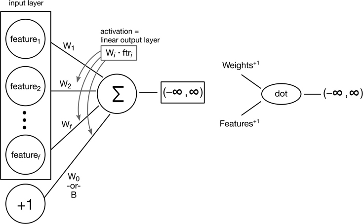
Figure 15.3 A neural network view of linear regression.
To implement that diagram, we are going to use a Python package called keras. In turn, keras is going to drive a lower-level neural network package called TensorFlow. Used together, they massively simplify the process of turning diagrams of neural network components into executable programs.
In [24]:
import keras.layers as kl
import keras.models as km
import keras.optimizers as ko
Using TensorFlow backend.
There are a number of ways to define and build a keras model. We’ll use a simple one that allows us to add layers to a model as we work forward—from left to right or from input to output. This process is sequential, so we have to keep moving strictly forward. Now, it turns out that classic linear regression only requires one work layer. This work layer connects the inputs and the outputs (which are layers in their own right, but we’re not concerned with them since they are fixed in place).
Back to the work layer: in Keras, we define it as a Dense layer. That means that we connect all of the incoming components together (densely). Further, we create it as a Dense(1) layer. That means that we connect all of the incoming components together into one node. The values funnel through that single node and form a dot product. That was specified when we said activation='linear'. If you’re getting a distinct feeling of linear regression déjà vu, you’re right. That’s exactly what we get.
The last piece in our model builder is how we’re going to optimize it. We have to define our cost/loss function and the technique we use to minimize it. We’ll use a mean-squared-error loss (loss='mse') and a rolling-downhill optimizer called stochastic gradient descent (ko.SGD). The gradient descent part is the downhill bit. The stochastic part means that we use only a part of our training data—instead of all of it—every time we try to figure out the downhill direction. That technique is very useful when we have a mammoth amount of training data. We use lr (learning rate) in the same way we used step_size in Section 15.1: once we know a direction, we need to know how far to move in that direction.
In [25]:
def Keras_LinearRegression(n_ftrs):
    model = km.Sequential()
    # Dense layer defaults include a "bias" (a +1 trick)
    model.add(kl.Dense(1,
                       activation='linear',
                       input_dim=n_ftrs))
    model.compile(optimizer=ko.SGD(lr=0.01), loss='mse')
    return model
The keras developers took pity on us and gave their models the same basic API as sklearn. So, a quick fit and predict will get us predictions. One slight difference is that fit returns a history of the fitting run.
In [26]:
# for various reasons, are going to let Keras do the +1 trick
# we will *not* send the `ones` feature
linreg_ftrs = linreg_ftrs_p1[:,0]

linreg_nn = Keras_LinearRegression(1)
history = linreg_nn.fit(linreg_ftrs, linreg_tgt, epochs=1000, verbose=0)
preds = linreg_nn.predict(linreg_ftrs)

mse = metrics.mean_squared_error(preds, linreg_tgt)

print("Training MSE: {:5.4f}".format(mse))
Training MSE: 0.0000
So, we took the training error down to very near zero. Be warned: that’s a training evaluation, not a testing evaluation. We can dive into the fitting history to see how the proverbial ball rolled down the cost curve. We’ll just look at the first five steps. When we specified epochs=1000 we said that we were taking a thousand steps.
In [27]:
history.history['loss'][:5]
Out[27]:
[328.470703125,
 57.259727478027344,
 10.398818969726562,
 2.2973082065582275,
 0.8920286297798157]
Just a few steps made a massive amount of progress in driving down the loss.
15.5.2 A NN View of Logistic Regression
The neural network diagrams for linear regression (Figure 15.3) and logistic regression (Figure 15.4) are very similar. The only visible difference is the wavy sigmoid curve on the logistic regression side. The only difference when we go to implement logistic regression is the activation parameter. Above, for linear regression, we used a linear activation—which, as I told you, was just a dot product. For logistic regression, we’ll use a sigmoid activation which basically pipes a dot product through a sigmoid curve. Once we put that together with a different loss function—we’ll use the log loss (under the name binary_crossentropy)—we’re done. In truth, we’re only done because the output here is a probability. We have to convert that to a class by comparing with .5.

Figure 15.4 A neural network view of logistic regression.
In [28]:
def Keras_LogisticRegression(n_ftrs):
    model = km.Sequential()
    model.add(kl.Dense(1,
                       activation='sigmoid',
                       input_dim=n_ftrs))
    model.compile(optimizer=ko.SGD(), loss='binary_crossentropy')
    return model

logreg_nn = Keras_LogisticRegression(1)
history = logreg_nn.fit(logreg_ftr, logreg_tgt, epochs=1000, verbose=0)

# output is a probability
preds = logreg_nn.predict(logreg_ftr) > .5
print('accuracy:', metrics.accuracy_score(preds, logreg_tgt))
accuracy: 0.92
15.5.3 Beyond Basic Neural Networks
The single Dense(1) layer of NNs for linear and logistic regression is enough to get us started with basic—shallow—models. But the real power of NNs comes when we start having multiple nodes in a single layer (as in Figure 15.5) and when we start making deeper networks by adding layers.

Figure 15.5 Dense layers.
Dense(1, "linear") can only perfectly represent linearly separable Boolean targets. Dense(n) can represent any Boolean function—but it might require a very large n. If we add layers, we can continue to represent any Boolean function, but we can—in some scenarios—do so with fewer and fewer total nodes. Fewer nodes means fewer weights or parameters that we have to adjust. We get simpler models, reduced overfitting, and more efficient training of our network.
As a quick example of where these ideas lead, the MNIST handwritten digit recognition dataset—similar to sklearn’s digits—can be attacked with a multiple working-layer neural network. If we string together two Dense(512) layers, we get a network with about 670,000 weights that must be found via optimization. We can do that and get about a 98% accuracy. The most straightforward way to do that ends up losing some of the “imageness” of the images: we lose track of which pixels are next to each other. That’s a bit like losing word order in bag-of-words techniques. To address this, we can bring in another type of network connection—convolution—that keeps nearby pixels connected to each other. This cuts down on irrelevant connections. Our convolutional neural network has only 300,000 parameters, but it can still perform similarly. Win-win. You can imagine that we effectively set 370,000 parameters to zero and have far fewer knobs left to adjust.
15.6 Probabilistic Graphical Models
I introduced neural networks as a graphical model: something we could easily draw as connections between values and operations. One last major player in the modern learning toolbox is probabilistic graphical models (PGMs). They don’t get quite the same press as neural networks—but rest assured, they are used to make important systems for image and speech processing and in medical diagnosis. I want to give you a quick flavor of what they are and what they get us over-and-above the models we’ve seen so far. As we did with neural networks, I’m going to show you what linear and logistic regression look like as PGMs.
Up to now, even with neural network, we considered some data—our input features and our targets—as a given and our parameters or weights as adjustable. In PGMs, we take a slightly different view: the weights of our models will also be given some best-guess form as an additional input. We’ll give our model weights a range of possible values and different chances for those values popping out. Putting these ideas together means that we are giving our weights a probability distribution of their possible values. Then, using a processes called sampling, we can take the known, given data that we have, put it together with some guesses as to the weights, and see how likely it is that the pieces all work together.
When we draw a neural network, the nodes represent data and operations. The links represent the flow of information as operations are applied to their inputs. In PGMs, nodes represent features—input features and the target feature—as well as possible additional, intermediate features that aren’t represented explicitly in our data. The intermediate nodes can be the results of mathematical operations, just like in neural networks.
There are some amazing things we can do with PGMs that we can’t necessarily do with the models we’ve seen so far. Those models were easy to think of, conceptually, as sequences of operations on input data. We apply a sequence of mathematical steps to the inputs and, presto, we get outputs. Distributions over features are even more flexible. While we might think of some features as inputs and output, using distributions to tie features together means that we can send information from a feature to any other feature in that distribution. Practically speaking, we could (1) know some input values and ask what the right output values are, (2) know some output values and ask what the right input values are, or (3) know some combinations of inputs and outputs and ask what the right remaining input and output values are. Here, right means most likely given everything else we know. We are no longer on a one-way street from our input features going to our target outputs.
This extension takes us quite a ways past building a model to predict a single output from a group of inputs. There’s another major difference. While I’m simplifying a bit, the methods we’ve discussed up until now make a single, best-guess estimate of an answer (though some also give a probability of a class). In fact, they do that in two ways. First, when we make a prediction, we predict one output value. Second, when we fit our model, we get one—and only one—best-guess estimate of the parameters of our model. We can fudge our way past some special cases of these limits, but our methods so far don’t really allow for it.
PGMs let us see a range of possibilities in both our predictions and our fit models. From these, if we want, we can ask about the single most likely answer. However, acknowledging a range of possibilities often allows us to avoid being overconfident in a single answer that might not be all that good or might be only marginally better than the alternatives.
We’ll see an example of these ideas in a minute, but here’s something concrete to keep in mind. As we fit a PGM for linear regression, we can get a distribution over the weights and predicted values instead of just one fixed set of weights and values. For example, instead of the numbers {m = 3, b = 2} we might get distributions {m = Normal(3, .5), b = Normal(2, .2)}.
15.6.1 Sampling
Before we get to a PGM for linear regression, let’s take a small diversion to discuss how we’ll learn from our PGMs. That means we need to talk about sampling.
Suppose we have an urn—there we go again with the urns—that we draw red and black balls from, placing each ball back into the urn after we recorded its color. So, we are sampling with replacement. Out of 100 tries, we drew 75 red balls and 25 black balls. We could now ask how likely is it that the urn had 1 red ball and 99 black balls: not very. We could also ask how likely is it that the urn had 99 red balls and 1 black ball: not very, but more likely than the prior scenario. And so on. Eventually we could ask how likely is that the urn had 50 red and 50 black balls. This scenario seems possible but not probable.
One way we could figure out all of these probabilities is by taking each possible starting urn—with different combinations of red and black balls—and performing many, many repeated draws of 100 balls from them. Then we could ask how many of those attempts led to a 75 red and 25 black result. For example, with an urn that contains 50 red and 50 black balls, we pull out 100 balls with replacement. We repeat that, say, a million times. Then we can count the number of times we achieved 75 red and 25 black. We do that repeated sampling process over all possible urn setups—99 red, 1 black; 98 red, 2 black; and so on all the way up to 1 red, 99 black—and tally up the results.
Such a systematic approach would take quite a while. Some of the possibilities, while strictly possible, might practically never occur. Imagine drawing (75 red, 25 black) from an urn with (1 red, 99 black). It might only happen once before the sun goes supernova. Nevertheless, we could do this overall process.
The technique of setting up all legal scenarios and seeing how many of the outcomes match our reality is called sampling. We typically don’t enumerate—list out—all of the possible legal scenarios. Instead, we define how likely the different legal scenarios are and then flip a coin—or otherwise pick randomly—to generate them. We do this many times so that, eventually, we can work backwards to which of the legal scenarios are the likely ones. Scenarios that are possible but not probable might not show up. But that’s OK: we’re focusing our efforts precisely on the more likely outcomes in proportion to how often they occur.
Our urn example uses sampling to determine the percent of red—and hence also the black—balls in the urn. We do assume, of course, that someone hasn’t added a yellow ball to the urn behind our backs. There’s always a danger of an unknown unknown. In a similar way, sampling will allow us to estimate the weights in our linear and logistic models. In these cases, we see the input and output features and we ask how likely this, that, or another set of weights are. We can do that for many different possible sets of weights. If we do it in a clever way—there are many, many different ways of sampling—we can end up with both a good single estimate of the weights and also a distribution of the different possible weights that might have led to the data we see.
15.6.2 A PGM View of Linear Regression
Let’s apply the idea of PGMs to linear regression.
15.6.2.1 The Long Way
Here’s how this works for our good old-fashioned (GOF) linear regression. We start by drawing a model (Figure 15.6) of how the features and weights interact. This drawing looks an awful lot like the model we drew for the neural network form of linear regression, with the addition of placeholder distributions for the learned weights.

Figure 15.6 A probabilistic graphical model for linear regression.
Our major tool for exploring PGMs is going to be pymc3. The mc stands for Monte Carlo, a famous casino. When you see that name, you can simply mentally substitute randomness.
In [29]:
import pymc3 as pm

# getting really hard to convince toolkits to be less verbose
import logging
pymc3_log = logging.getLogger('pymc3')
pymc3_log.setLevel(2**20)
For most of the book, we’ve swept this detail under the carpet—but when we predict a value with a linear regression, we have really been predicting a single output target value that is a mean of the possible outcomes at that spot. In reality, if our data isn’t perfect, we have some wiggle room above and below that value. This possible wiggle room—which GOF linear regression treats as the same for each prediction—is a normal distribution. Yes, it really does show up everywhere. This normal distribution is centered at the predicted value with a standard deviation around that center, so it shows up as a band above and below our linear regression line. Our predictions still fall on the linear regression line. The new component is simply something like a tolerance band around the line. When we look at linear regression as PGM, we make this hidden detail explicit by specifying a standard deviation.
Let’s turn our diagram from Figure 15.6 into code:
In [30]:
with pm.Model() as model:
    # boilerplate-ish setup of the distributions of our
    # guesses for things we don't know
    sd        = pm.HalfNormal('sd', sd=1)
    intercept = pm.Normal('Intercept', 0, sd=20)
    ftr_1_wgt = pm.Normal('ftr_1_wgt', 0, sd=20)

    # outcomes made from initial guess and input data
    # this is y = m x + b in an alternate form
    preds = ftr_1_wgt * linreg_table['ftr_1'] + intercept

    # relationship between guesses, input data, and actual outputs
    # target = preds + noise(sd) (noise == tolerance around the line)
    target = pm.Normal('tgt',
                       mu=preds, sd=sd,
                       observed=linreg_table['tgt'])

    linreg_trace = pm.sample(1000, verbose=-1, progressbar=False)
After all that, not seeing any output is a bit disappointing. Never fear.
In [31]:
pm.summary(linreg_trace)[['mean']]
Out[31]:
|
mean |
|---|---|
Intercept |
2.0000 |
ftr_1_wgt |
3.0000 |
sd |
0.0000 |
Now that is comforting. While we took a quite different path to get here, we see that our weight estimates are 3 and 2—precisely the values we used to generate the data in linreg_table. It’s also comforting that our estimate as to the noisiness of our data, sd, is zero. We generated the data in linreg_table without any noise. We are as perfect as we can be.
15.6.2.2 The Short Way
There are a lot of details laid out in that code example. Fortunately, we don’t have to specify each of those details every time. Instead, we can write a simple formula that tells pymc3 that the target depends on ftr_1 and a constant for the +1 trick. Then, pymc3 will do all the hard work of filling in the pieces we wrote out above. The family= argument serves the same role as our target= assignment did in our long-hand version. Both tell us that we are building a normal distribution centered around our predictions with some tolerance band.
In [32]:
with pm.Model() as model:
    pm.glm.GLM.from_formula('tgt ~ ftr_1', linreg_table,
                            family=pm.glm.families.Normal())
    linreg_trace = pm.sample(5000, verbose=-1, progressbar=False)
pm.summary(linreg_trace)[['mean']]
Out[32]:
|
mean |
|---|---|
Intercept |
2.0000 |
ftr_1 |
3.0000 |
sd |
0.0000 |
The names here are the names of the features. I’d be happier if it was clear that they are the values of the weights on those features. Still, consider my point made. It’s reassuring that we get the same answers for the weights. Now, I brought up a benefit of PGMs: we can see a range of possible answers instead of just a single answer. What does that look like?
In [33]:
%%capture

# workaround for a problem: writing to a tmp file.
%matplotlib qt

fig, axes = plt.subplots(3,2,figsize=(12,6))
axes = pm.traceplot(linreg_trace, ax=axes)
for ax in axes[:,-1]:
    ax.set_visible(False)

plt.gcf().savefig('outputs/work-around.png')
In [34]:
Image('outputs/work-around.png', width=800, height=2400)
Out[34]:
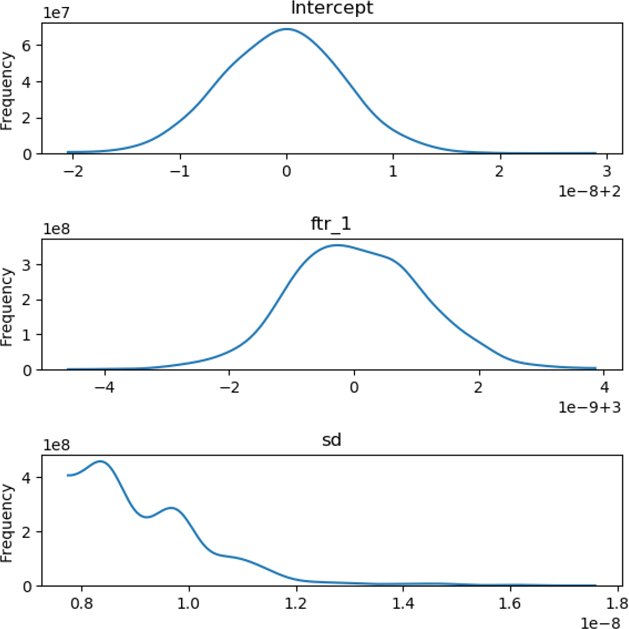
These graphs may be hard to read because the units are a bit wacky, but 1e-8 and 1e-9—one times ten to the minus eight and nine—are both approximately zero. So, those labels in the bottom right (the scale of the x-axis) are really funky ways of saying that the centers of the graphs are 2 and 3, exactly the values we saw in the previous table. The sd values are just little pieces sized like 1e-8—again, pretty close to zero. Good. What we see with the big bumps is that there is a highly concentrated area around the values from the table that are likely to have been the original weights.
15.6.3 A PGM View of Logistic Regression
Having seen the close relationships between linear and logistic regression, we can ask if there is a similarly close relationship between PGMs for the two. Unsurprisingly, the answer is yes. Again, we need only a tiny change to go from linear regression to logistic regression. We’ll start by looking at a diagram for the PGM in Figure 15.7.

Figure 15.7 A probabilistic graphical model for logistic regression.
We can spin up almost the exact same model as linear regression except with a slightly different family: now we need to use Binomial as our target. Whenever you see binomial, you can immediately use a mental model of coin flipping. Since our logistic regression example has two classes, we can think of them as heads and tails. Then, we are simply trying to find the chances of flipping a head. Making that substitution—of the binomial distribution for the normal distribution—gives us the following code:
In [35]:
with pm.Model() as model:
    pm.glm.GLM.from_formula('tgt ~ ftr_1', logreg_table,
                            family=pm.glm.families.Binomial())
    logreg_trace = pm.sample(10000, verbose=-1, progressbar=False)
pm.summary(logreg_trace)[['mean']]
Out[35]:
|
mean |
|---|---|
Intercept |
22.6166 |
ftr_1 |
-2.2497 |
Our results here are not exact: the true, original values were 20 and –2. But remember, our logreg_table was a bit more realistic than our linear regression data. It included noise in the middle where examples were not perfectly sorted into heads and tails—our original zeros and ones.
For linear regression, we looked at the univariate—stand-alone—distributions of the weights. We can also look at the bivariate—working together—distributions of the weights. For the logistic regression example, let’s see where the most likely pairs of values are for the two weights.
In [36]:
%matplotlib inline

df_trace = pm.trace_to_dataframe(logreg_trace)
sns.jointplot('ftr_1', 'Intercept', data=df_trace,
              kind='kde', stat_func=None, height=4);

The darker area represents the most likely combinations of weights. We see that the two are not independent of each other. If the weight on ftr_1 goes up a bit—that is, becomes a little less negative—the weight on the intercept has to go down a bit.
You can think of this like planning for a long drive. If you have a target arrival time, you can leave at a certain time and drive at a certain speed. If you leave earlier, you can afford to drive a bit more slowly. If you leave later—holiday craziness, I’m looking at you—you have to drive more quickly to arrive at the same time. For our logistic regression model, arriving at the same time—the dark parts of the graph—means that the data we see is likely to have come from some tradeoff between the start time and the driving speed.
15.7 EOC
15.7.1 Summary
We’ve covered three main topics here: (1) how several different learning algorithms can be solved using generic optimization, (2) how linear and logistic regression can be expressed using neural networks, and (3) how linear and logistic regression can be expressed using probabilistic graphical models. A key point is that these two models are very close cousins. A second point is that all learning methods are fundamentally doing similar things. Here’s one last point to consider: neural networks and PGMs can express very complicated models—but they are built from very simple components.
15.7.2 Notes
If you are interested in learning more about optimization, take a glance at zero-finding and derivatives in a calculus class or dig up some Youtube videos. You can get entire degrees in finding-the-best. There are people studying optimization in mathematics, business, and engineering programs.
Logistic Regression and Loss With z = βx, probability in a logistic regression model is . That also gives us p = logistic(z) = logistic(βx). Minimizing the cross-entropy loss gives us these expressions:
For 0/1: –yz + log(1 + ez)
For ±1: log(1 + e–yz)
When we go beyond a binary classification problem in NN, we use a one-hot encoding for the target and solve several single-class problems in parallel. Then, instead of using the logistic function, we use a function called softmax. Then, we take the class that results in the highest probability among the possible targets.
Neural Networks It’s really hard to summarize the history of neural networks in four sentences. It started in the mid-1940s and had a series of boom-bust cycles around 1960 and then in the 1980s. Between the mid-1990s and early 2010s, the main theoretical and practical hardware problems got workable solutions. For a slightly longer review, see “Learning Machine Learning” by Lewis and Denning in the December 2018 issue of the Communications of the ACM.
I mentioned briefly that we can extend neural networks to work with more than binary target classification problems. Here’s a super quick example of those techniques applied to a binary problem. You can adjust the number of classes to work with larger problems simply by increasing n_classes.
In [37]:
from keras.utils import to_categorical as k_to_categorical
def Keras_MultiLogisticRegression(n_ftrs, n_classes):
    model = km.Sequential()
    model.add(kl.Dense(n_classes,
                       activation='softmax',
                       input_dim=n_ftrs))
    model.compile(optimizer=ko.SGD(), loss='categorical_crossentropy')
    return model

logreg_nn2 = Keras_MultiLogisticRegression(1, 2)
history = logreg_nn2.fit(logreg_ftr,
                         k_to_categorical(logreg_tgt),
                         epochs=1000, verbose=0)

# predict gives "probability table" by class
# we just need the bigger one
preds = logreg_nn2.predict(logreg_ftr).argmax(axis=1)
print(metrics.accuracy_score(logreg_tgt, preds))
0.92
15.7.3 Exercises
Can you do something like
GridSearch—possibly with some clunky looping code—with our manual learning methods to find good values for our regularization controlC?We saw that using a penalty on the weights can actually hurt our weight estimates, if the data is very clean. Experiment with different amounts of noise. One possibility is bigger spreads in the standard deviation of regression data. Combine that with different amounts of regularization (the
Cvalue). How do our testing mean-squared errors change as the noise and regularization change?Overfitting in neural networks is a bit of an odd puppy. With more complicated neural network architectures—which can represent varying degrees of anything we can throw at them—the issue becomes one of controlling the number of learning iterations (epochs) that we take. Keeping the number of epochs down means that we can only adjust the weights in the network so far. The result is a bit like regularization. As you just did with the noise/
Ctradeoff, try evaluating the tradeoff between noise and the number of epochs we use for training a neural network. Evaluate on a test set.