CHAPTER 3

Individual Equilibrium

The title of this chapter might seem puzzling to the reader. In Chapter 1, we distinguished macroeconomics from microeconomics by defining the former as applying to aggregate economic activity and the latter to individual economic activity.

Yet, macroeconomic activity boils down to decisions to supply labor and financial capital (which is what people provide when they save) to firms that use their labor and financial capital to produce the goods that workers buy. This means that we have go through some microeconomics before aggregating the choices made at the microlevel to the entire economy.

So let’s start with some fundamentals: Firms produce things because individuals are willing to supply them with labor and financial capital. People supply labor because the reward for doing so, as measured by their after-tax earnings, exceeds the reward for not doing so, as measured by forgone pleasures of leisure and as affected by the numerous incentives government offers to people not to work.

People save because the after-tax return they receive for putting their cash into financial instruments like bank certificates of deposits (CDs) and corporate stocks exceeds the pleasures of using that cash for current consumption. Their incentives to save are, as we shall see, diminished by taxes on capital income.

This chapter and the next will work through the details of what determines people’s willingness to work and save. Once we have the groundwork in place for determining how people choose to work and save, we will then consider how firms take their work and saving and convert it into production.

Why Am I Writing This Book?

At any moment, I have a choice between working and not working. At this moment I am writing the book in front of you. In the parlance of economics, I am sacrificing leisure and, in the process, supplying labor services in exchange for what I hope to be the income (and satisfaction) that I will enjoy several months from this moment when the book is published. Maybe I will apply the future income I get from writing the book toward the purchase of a car. Or maybe I will use it to acquire financial assets that I will need to fund my eventual retirement. In the first instance, and on the basis of narrow pecuniary considerations, I would use the income to finance current consumption and, in the second, again in the parlance of economics, to finance future consumption or leisure.

Suppose, on the other hand, that instead of writing this book, I were engaged in a consulting project for which I was paid as I worked. The consulting assignment would pay a fixed, agreed-upon amount immediately, not a royalty contingent on book sales. So which is the better choice? The book or the consulting project?

The fact is that either pursuit—the book or the consulting project— would require the sacrifice of current leisure so that I might as well choose the project (the book) from which I would get more personal satisfaction, no matter what pecuniary reward I might get. Thus the choice of the book-writing project became the superior one in my personal calculus.

Yet, I did perform a cost-benefit test before committing to it. It was a matter of making choices at the margin: the sacrifice of some certainty and an immediacy of rewards in exchange for personal satisfaction and the hope that the future rewards from the book will exceed the current rewards from any other use of my time.

I make these reflections, not because I think they will fascinate the reader, but because of how obvious they must seem, once revealed. Every person in every day of his or her life makes choices like the one I did. You might ask yourself: Shall I double down at the office and work all the harder in hopes of a promotion, or shall I take the time to polish my resume and start looking for something better? Shall I take a part-time job now that the kids are in high school and make the needed investment in new clothes and maybe a new car, or shall I go back to school or just stay at home until they are in college?

The government presents us with other less appealing choices. Shall I take another job and boost my income or just let well enough alone and avoid disqualifying my family from health care subsidies or unemployment insurance? Shall I take the higher paying job on the other coast or avoid uprooting my family and pushing us into a higher tax bracket? Shall I save more now or believe the government’s promises about future Social Security benefits? How about that stock tip from my broker? Should I buy the stock or not, considering that the tax on corporate income has just gone down, or just put the money in a low-paying but safe CD?

Such choices, as they are made every day by every participant in the economic system, give rise to the activity we study under the heading of macroeconomics. Yes, when we assess or predict the performance of the “macroeconomy,” we look at broad indices of how individual choices combine to produce overall economic activity, but behind those indices are minute choices of the kind just described in which people make trade-offs between the different uses of their time and money.

Macroeconomists, as noted in the Introduction, look at the big trade-offs, and not the small ones. We look at the total number of hours available to the age-eligible population and think about how that population divides those hours between work and leisure. We look at national income and think about how the country divides what’s left of that income after taxes between consumption and saving. We think big.

But we also think small. That’s because, as noted before, all the big choices are the result of small choices by individuals about how to divide their time between work and leisure and how to divide their after-tax income between consumption and saving. Thus we have to drill down to the choice calculus of the individual who must decide how to spend each day as it looms ahead of him at 5:00 a.m. (I’m an early riser) and how to use each paycheck that appears (minus the part that goes to government) each month in his bank statement.

That is the way macroeconomists of the new classical persuasion approach their subject, and that is the way we approach macroeconomics in this chapter.

Oh, and one more thing. This chapter and the next embrace what macroeconomists call a microfoundations approach: working up to the big from the small. A characteristic of this approach is that it makes use of a hypothetical individual called the “representative agent.” In this book, to avoid worrying my editors in an age of gender sensitivity, I have two representative agents: Adam and Eve. I rely on Biblical authority to start with Adam, but after he has been expelled from Eden and faces the necessity of making worldly trade-offs.

So let’s begin with the problem faced by Adam when it comes to supplying his labor services. There are 24 hours in a day, 168 hours in a week, and 8,760 hours in a year. Adam, whom we assume to be 16 or older and not in prison (i.e., a member of the age-eligible population), must spend every one of those hours either working for money or not working for money. Economists, as previously stated, characterize this as a choice between work and leisure even if time counted as leisure includes going to college, cutting the lawn, or any other activity, however pleasurable or onerous, that is not directed at making money. (We ignore barter as offering the option of gains from trade without the need for money.)

The reader may think it strange to imagine a worker carefully deciding every day, week, or year how much time to allocate between work and leisure. Shall Adam work eight hours today? Or six? Or 16? Twelve months this year or only three? In fact, there are many occupations that provide flexibility in choosing working hours. And there are workers with eight-hour-a-day jobs who choose to work part time at other jobs. And many workers move in and out of eight-hour-a-day and temporary jobs over the course of their lifetimes.

In deciding how to divide his time between work and leisure, Adam has to take into account how his current choices will affect his future choices. If he makes $100 by working an hour today, he could spend the entire amount today or use the $100 to buy some income-earning asset and then use the cash value of that asset to engage in consumption at a later time. Or he could enjoy leisure and put off work to the future.

The Labor—Leisure Choice

Let’s suppose that Adam has just two periods to live: period 1 and period 2. Period 1 starts on a given day at midnight and period 2 is the day that begins a year later at midnight. (It is as if, Adam comes back to life in a year, in a manner reminiscent of Rip Van Winkle.) The period-1 wage rate is w₁, and the period-2 wage rate is w₂. In period 1, Adam has h hours available to divide between leisure and labor. (Because we will usually think in terms of the labor-leisure choice over a single day, h is taken to equal 24.) Let’s abbreviate period-1 labor income as lay₁ (This follows the convention of using the letter y to designate income, in this instance labor income, and lower-case letters to represent individual rather than societal choices.) Then

where le₁ is the amount time Adam allocates to leisure in period 1, so that if le₁ = 16, he works eight hours that day. (There are no taxes to worry about just yet. We postpone that worry to future chapters.)

We can write a similar equation for lay₂, his period-2 labor income:

Adam can receive income in the form of wages (sometimes called “earned income”) or in the form of income on some asset that he owns, such as a bank CD (“unearned income” or asset income). For now let’s assume that Adam’s total period-1 income y₁ is labor income, so that

but that he can receive asset income as well as labor income in period 2. Adam can receive a return of r on an asset that he purchases out of his saving sav₁ in period 1. He then divides his period-1 income between consumption c₁ and saving sav₁, so that

Now we can write an equation for his total income in period-2 as

Note that y₂ has three parts: (a) Adam’s period-2 labor income, lay₂, his period-2 interest income, r × sav₁, and his income, sav₁, from the sale of the asset he bought in period 1. In this thought experiment, we have to imagine that Adam thinks in terms of how his saving on May 1, 2018, will contribute to his income on May 1, 2019.

So far, because labor income depends on the division of time between labor and leisure, Adam has three variables, le₁, le₂, and sav₁, for which to solve in order to determine his total income in period 1 and period 2.

Substituting equation (3.4) into equation (3.5), we get

Because the individual thinks only in terms of the two periods, we assume that he will not save in period 2. Thus that part of his period-2 consumption that is affected by his period-1 choices will be equal to his period-2 labor income plus however much he saved in period 1 plus the return on his saving. Think of Adam as buying an IOU in period 1 for which he pays sav₁ and then sells the IOU just before it matures in period 2 for sav₁(1 + r). That becomes his income from saving. His period-2 consumption then is

Rearranging,

The left-hand side of this equation represents the present value of Adam’s current and future consumption and the right-hand side the present value of his current and future labor income. The equation illustrates the principle that at every moment in our lives we are making a choice between current and future consumption based on expectations about our current and future income. To understand this, let’s get a firm idea of what is meant by “present value.”

Suppose that r = 10%, lay₁ = $500, and lay₂ = $550. Then the present value of Adam’s labor income is $1,000. The present value of lay₁ is $500 because that is the money that he will receive during the current period. The present value of the $550 to be received a year from now is, at 10% interest, also $500

To see what this means, suppose that Adam wants to spend $1,000 in period 1. He has only $500 in income in that period, so in order to spend $1,000 in period 1, he must borrow against his period-2 labor income. Because the interest rate is 10%, he would have to borrow $500 now and pay back principal and interest of $550 out of his period-2 income. If he takes this route, he is left with no money to apply to consumption in period 2. Or Adam could, at the other extreme, consume nothing in period 1, put his period-1 income in the bank, so that with interest he would have $550 to apply to his period-2 consumption, permitting him to set his period-2 consumption at $1,100.

Now let’s rewrite equation (3.8) as follows:

This tells us that labor income in period 1 can be used to finance period-1 consumption or period-2 consumption, or to reduce period-2 labor income and thus period-2 work time. Conversely, period-2 labor income can be used to finance period-1 consumption or period-2 consumption, or to reduce period-1 labor income and thus period-1 work time. Everything depends on everything else.

But how does Adam make these trade-offs? Let’s approach this question by assuming for now that, in choosing lay₁, Adam takes lay₂ as fixed and that in choosing lay₂ he takes lay₁ as fixed. (We will relax that assumption later on.)

We also need some assumptions about how Adam chooses between labor income and leisure. Most fundamentally, we assume that Adam wants to maximize utility. In Chapter 4 we will discuss the idea of maximizing the present value of a utility function, which is defined over consumption that takes place for an entire lifetime. Here we keep things simple by sticking with the two-period example.

Let’s first think of our decision-maker Adam as having to choose between more or less leisure now. Suppose Adam has been dividing his day between 10 hours of work and 14 hours of leisure and that he has been making $500 per day in income. Now he considers expanding his leisure by one hour. The question is how much income, at most, would he be willing to sacrifice for that additional hour of leisure?

In considering a problem like this we can imagine that Adam carries a computer around in his head, which assigns units of utility—utiles—to different quantities of things. This brain computer assigns a certain number of utiles to Adam’s leisure time and certain number to his income. For now, we don’t have to care about Adam’s total utility from leisure and income. All we have to care about is his marginal utility of leisure and of labor income. The marginal utility of leisure is the change in utility that Adam experiences per unit change in leisure, which can be written as Suppose, for example, that an additional hour of leisure would increase Adam’s utility by 400 utiles. Then we would write:

which is to say that the change in Adam’s utility per unit change in leisure is 400. We see Adam choosing leisure time in terms of hours. So one more hour of leisure adds 400 to Adam’s total utility.

Now let’s ask about the marginal utility of his labor income. Let’s suppose that the following equation applies:

which means that the change in his utility per unit change in labor income is 4. One more dollar of labor income adds 4 units of utility. Labor income adds to utility because it makes it possible to consume more, now or later.

Proceeding with this example, the question is how much income, at most, would Adam be willing to give up for an additional hour of leisure? The answer is $100. Why? To show why (if it isn’t already obvious) we introduce another concept, which we will call the marginal rate of substitution of leisure for labor income (MRS_LeLay). We can define the MRS_LeLay as which indicates the amount of labor income the individual is willing to give up for another unit of leisure or, equivalently, the amount of labor income with which the individual must be compensated to be willing to give up a unit of leisure. In this example, the MRS_LeLay is $100 ¹

We assume that utility rises with a rise in both leisure and income, so that the individual always prefers more leisure to less leisure and more income to less income. Thus, in Figure 3.1, where we measure Adam’s leisure along the horizontal axis and his labor income along the vertical axis, he prefers the combination of leisure and labor income indicated by point X to that indicated by point Y₁ and that to point Z.

Just as Adam always prefers more to less, in this fashion, he can be indifferent between combinations like Y₁ and Y₂, where one combination has more income than the other, but less leisure, or more leisure but less income. A curve that traces out these combinations is called an indifference curve, and it indicates different combinations of leisure and labor income that register a fixed amount of utility in Adam’s brain computer.

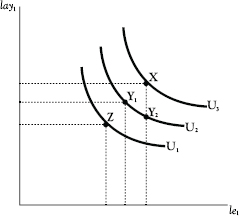
Figure 3.1 Individual indifference curves for leisure and labor income

Figure 3.1 contains three such indifference curves, all of which have some properties in common: (1) they are negatively sloped, to reflect the idea that for Adam to remain at the same level of utility, he has to give up some leisure as income expands, (2) they do not intersect (which is necessary for his choices to be consistent), and (3) they are bulged downward, that is, “convex.” Adam’s total utility rises as he moves from indifference curve U₁ to indifference curve U₂ to indifference curve U₃ but constant as he moves along any of these curves.

Now our job is to lay out a process by which Adam makes his leisure-work choices in period 1. We begin by assuming that work becomes more onerous, and leisure more desirable as more and more time is allocated to work. A person who is working 14 hours a day, and has only 10 hours a day for sleep and other “leisure” activities, would be willing to give up quite a bit of labor income for another hour of leisure, whereas a person who is working four hours a day, and already has 20 hours of leisure, would be willing to give up only a little labor income for an extra hour of leisure. Hence, the downward bulge in the indifference curves. Let’s illustrate, beginning with the same example we just considered.

See Figure 3.2. If Adam is at point X₁ on one of his indifference curves, he is consuming 10 hours of leisure and getting $700 per day in income. Now he considers expanding his leisure from 10 to 11 hours, so that he would move from point X₁ to point X₂. We see that he can sacrifice as much as $100 in income in making this move without moving to a lower level of utility. Now compare a possible move from X₃ to X₄. Once Adam has expanded his leisure time to 14 hours per day, he is willing to give up only as much as $25 in labor income for another hour of leisure.

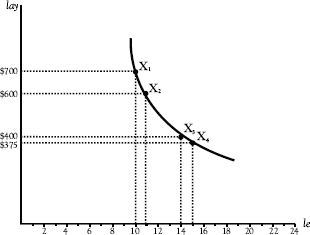
Figure 3.2 Declining MRS_LeLay

Adam’s MRS_LeLay is $100 when he has 10 hours a day in leisure and $25 when he has 14 hours a day in leisure. His choices are governed by the law of diminishing marginal rate of substitution of leisure for labor income, whereby the amount of labor income he is willing to give up for an hour of leisure falls as leisure increases. Equivalently, the amount of labor income with which he must be compensated in order to give up an hour of leisure decreases as his leisure expands.

Figure 3.3 shows how Adam picks the combination of consumption and leisure that maximizes his utility, that is, leaves him in the best position. Here we assume that he gets a wage of $50 per hour, as measured by the slope of the line CD, and that he has to decide how to allocate his time each day between consumption and leisure. If he wanted to, he could (technically at least) have either (1) $1,200 in labor income and no leisure or (2) no labor income and 24 hours of leisure or any linear combination in between.

In this example, Adam picks point X₂ where he makes $500 in wages, allocating 10 hours of his day to work and 14 hours to leisure. Why X₂? The answer is that any other point on CD would leave him worse off.

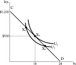
Figure 3.3 Individual equilibrium in the leisure and income choice calculus

First, Adam will not pick points X₁ or X₃ because they lie on an indifference curve U₁, which lies below the indifference curve U₂ on which X₂ is located. We can see this also if we measure the marginal rate of substitution as the absolute value of the slope of the indifference curve, wherever we find ourselves along an indifference curve on line CD.² We would expect indifference curves to be steep for combinations of leisure and labor income that contain a small amount of leisure and large amount of labor income and to be flat for combinations that contain a large amount of leisure and a small amount of labor income. Thus, the indifference curve for U₁ is steeper at point X₁ on CD than it is at X₃.

At point X₁, Adam is willing to give up more than $50 in labor income for another unit of leisure, as measured by the slope of indifference curve U₁ at that point. Because it costs only $50 in foregone wages and consumption for an additional unit of leisure, he will increase utility by moving down CD toward point X₂.

At points to the right of X₂, Adam is willing to give up less than $50 in labor income for an additional hour of leisure. At point X₃, for example, the last hour of leisure enjoyed was worth less than $50, as evidenced by the flatness of the curve. Adam will want to move back up CD to point X₂. Thus the optimal choice of consumption and leisure is represented by point X₂. It is at this point that the slope of his highest attainable indifference curve U₂ is just equal to the slope of line CD, which equals $50. Because, at this point,

Adam cannot increase his utility by either reducing or increasing the amount of leisure he enjoys.

Now let’s examine Adam’s period-2 calculus and in combination with his period-1 calculus just described. We represent this in Figure 3.4. Panel (a) presents the same information as Figure 3.3, except that the vertical axis is now the leisure axis and the horizontal axis is the labor income axis. (By flipping the axes in this figure, we can observe the combined results of his period-1 and period-2 choices.) Panel (b) illustrates Adam’s period-2 choices, with the horizontal axis serving as the leisure axis and the vertical axis as the labor income axis, as before. We assume that he expects his period-2 wage rate to be $55 per hour. Adam (coincidentally) chooses to allocate 10 hours to work and 14 hours to leisure in both period 1 and period 2. His period-2 labor income is $550. In equilibrium,

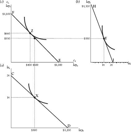
Figure 3.4 The two-period choice calculus

Panel (c) illustrates the choice faced by Adam in choosing between period-1 and period-2 consumption. Assume that there is an interest rate of 10%, which Adam receives on any money he saves and which he pays on any money he borrows. He can then have as much as $1,000 in period-1 consumption, and $0 in period-2 consumption, if he wishes, or $0 in period-1 consumption and $1,100 in period-2 consumption or any linear combination of these choices.

The Consumption—Saving Choice

Let’s see how these choices present themselves. We have already seen how Adam could end up with $1,000 in period-1 consumption and $0 in period-2 consumption. In this event, he simply consumes all of his period-1 income, which comes to $500. Then he borrows money from the bank (or maybe his trusting brother-in-law) for $500, promising to pay $500 plus interest of $50 when the loan comes due. That will leave him with $1,000 to consume in period 1 but nothing to consume in period 2. We can think of this as a process in which Adam sells an IOU to a lender and then pays off the IOU a year later.

Alternatively, Adam could use all of the $500 of current income to buy an IOU and then, when the IOU comes due in a year, supplement his period-2 labor income with the $550 principal and interest from the IOU to finance $1,100 in consumption. Line FE in Figure 3.5 illustrates these and all the intermediate possibilities. As in our earlier example, the present value of Adam’s period-1 and period-2 labor income is $1,000:

where indicates the equilibrium choice of labor income in period 1, and indicates the equilibrium choice of labor income in period 2.

The future worth of Adam’s period-1 and period-2 labor income is $1,100:

The slope of FE equals 1.1, reflecting the fact that Adam foregoes $1.10 [= $1(1 + r)] in consumption in the next period for each $1 he puts into consumption in this period. We say that the opportunity cost of $1 in consumption in this period is $1.10 in consumption in the next period.

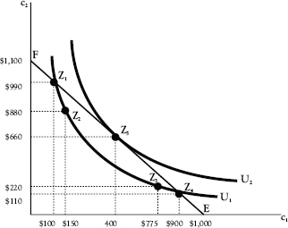
Figure 3.5 Individual equilibrium in the two-period consumption model

Adam has a utility-maximization problem in having to choose between current and future consumption. A dollar allocated to current consumption is a dollar not saved and a dollar not saved is a dollar plus earnings that is unavailable for future consumption. So the question is how the utility gained by adding a dollar to current consumption compares to the utility foregone by virtue of the resulting loss of future consumption. Let’s write the marginal utility of period-1 and period-2 consumption as follows:

where is the change in period-1 utility per dollar change in period-1 consumption, and is the change in period-2 utility per dollar change in period-2 consumption.

Part of the answer to the question just posed lies in the size of these variables: Insofar as the marginal utility of period-2 consumption exceeds the marginal utility of period-1 consumption, the individual is advised to shift consumption from period 1 to period 2.

Another consideration has to do with how Adam weighs period-2 utility against period-1 utility. We assume that he always puts the higher weight on current, or here, period-1 utility, than on future, or period-2, utility. We use ρ (the Greek letter rho) to indicate the amount of period-2 utility with which Adam must be compensated in order to willingly give up a unit of period-1 utility. We call ρ his rate of time preference. Thus the present value of period-1 plus period-2 utility is

which, in plain English, means that the value now of Adam’s current utility combined with his future utility is his current utility plus his future utility discounted by his rate of time preference. Then his marginal rate of substitution of current for future consumption is

Suppose that Adam’s period-1 utility rises by 200 utiles if he gets another dollar of period 1 consumption so that

and suppose that his period-2 utility rises by 105 utiles if he gets another dollar of period-2 consumption, so that

Finally suppose that his rate of time preference is 5%, meaning that, for Adam, a utile now is worth 5% more than a utile later.

This permits us to think about how the present value of Adam’s utility changes with his period-1 and period-2 consumption. The change in the present value of his marginal utility per unit change in period-1 consumption is

And the change in the present value of his marginal utility per unit change in period-2 consumption is

Then the marginal rate of substitution of c₁ for c₂ is

Adam is willing to give up $2 of period-2 consumption for $1 of period-1 consumption.

In Figure 3.5 we represent Adam’s preferences with indifference curves that have the same properties as the indifference curves presented in Figures 3.1 and 3.2. Each indifference curve reflects a higher level of utility than the indifference curves below it. Each has the familiar downward slope and a convex shape. And each has a property similar to the indifference curves just considered in examining the choice between leisure and labor income. This property is the diminishing marginal rate of substitution of period-1 consumption for period-2 consumption.

Line FE in the diagram represents the choices before Adam, given that he has $1,000 that he could spend now and given that he could have $1.10 in future consumption for every dollar that he saves now, which implies that r = 10%. Alternatively, we can say that Adam gives up $1.10 in period-2 consumption for every dollar he allocates to period-1 consumption.

Thus, if Adam spent the entire $1,000, he would have nothing to spend in period 2. If he spent only $100 now and saved the remaining $900, he would have $990 to spend in period 2, and so forth.

Suppose Adam chooses point Z₁, where his period-2 consumption would be $990, and considers expanding his period-1 consumption from $100 to $150. We see, from curve U₁, that he would remain at the same level of satisfaction if he reduced his period-2 consumption to $880 and shifted to point Z₂. There he would consume $150 worth of goods in period 1 and $880 in period 2. We can calculate his marginal rate of substitution of period-1 for period-2 consumption approximately as

Adam is willing to give up, on the average, $2.20 of period-2 consumption for another dollar of period-1 consumption as he shifts from Z₁ to Z₂. But he has to give up only $1.10 in period-2 consumption in order to add another dollar to his period-1 consumption. Knowing this, he would want to expand his period-1 consumption. As he keeps expanding his period-1 consumption he would be willing to give up less and less of period-2 consumption for an extra dollar of period-1 consumption.

Now suppose Adam moves from Z₂ to Z₃. At Z₃, he consumes $775 in period 1 and $220 in period 2. His marginal rate of substitution is now approximately 1.06 (=$660/$625). He has expanded his period-1 consumption too far if he adjusts to point Z₃, in that he was willing to sacrifice, on average, adjusting from point Z₂ to point Z₃ only $1.06 of future consumption for another dollar of current consumption, whereas again, every dollar of current consumption that he enjoys costs him $1.10 in future consumption. The mistake grows worse if he shifts all the way to Z₄, in that the marginal rate of substitution has fallen still further and now equals 0.88 (=$110/$125). He was willing to give up only $0.88 in future consumption for another dollar of present consumption, whereas the future cost of that dollar of present consumption was, again, $1.10. He would want to move up line FE, expanding his period-2 consumption and contracting his period-1 consumption.

Adam can adjust to any point he wishes along the line FE but chooses the point that permits him to attain the highest indifference curve with a point in common with that line. As before, we can measure the at any point along an indifference curve by finding the slope of the indifference curve at that point. We see that he would maximize utility by adjusting to point Z₅, where the slope of curve U₂ just equals the slope of FE. There his marginal rate of substitution also just equals 1 + r = 1.10.

The concept of diminishing MRS_c1c2 is important for the discussion in Chapter 5 of capital formation. The MRS_c1c2 equals the amount of future consumption the individual is willing to forego for another dollar of current consumption. As the individual expands current consumption and thus decreases current saving, the amount of future consumption he is willing to forego for another dollar of current consumption declines. But the MRS_c1c2 can also be interpreted as the amount of future consumption with which the individual must be compensated in order to forego another dollar of current consumption. The other side of the coin is that the MRS_c1c2 rises as current consumption decreases and current saving rises.

This means that a business that seeks financial capital in order to engage in investment must offer a high enough reward to induce the saving needed to provide that financial capital. When Adam saves, he creates financial capital. He does that if he puts his saving in the bank, so that the bank can lend to a customer, or if he buys stock in a corporation. He even creates financial capital if he puts his saving in a cookie jar, perhaps as a buffer against future emergencies.

Putting the Choices Together

Now return to Figure 3.4. As mentioned previously, Adam’s period-1 wage rate is $50. See panel (a). His period-2 wage rate is $55, as shown in panel (b). The decision to have 14 hours of daily leisure in both period 1 and period 2 translates into $500 in period-1 labor income and $550 in period-2 labor income. The decision to have $400 in period-1 consumption then translates into a decision to have $660 in period-2 consumption: Our decision maker, Adam, consumes $400 of his $500 in period-1 labor income, saving $100. He then augments his period-2 consumption with $110 in spending, as he cashes in the asset that he bought for $100 in period 1, which is now, at 10% interest, worth $110. In this way, he can set his period-2 consumption at $660.

Figure 3.6 illustrates how a change in the wage rates for period-1 and period-2 can affect these choices. In panel (a), Adam’s period-1 wage rate has risen from $50 to $70. In panel (b), his period-2 wage rate has fallen from $55 to $50. Period-1 leisure falls from 14 to 12 hours and thus work expands from 10 to 12 hours. Conversely, the fall in his period-2 wage rate causes him to expand leisure from 14 to 16 hours and to contract work from 10 to 8 hours.

In panel (c), the budget line FE, imported from Figure 3.4, correspondingly shifts outward in a manner parallel to itself so that it now becomes line F′E′, intersecting the horizontal axis at $1,204 and the vertical axis at $1,324. We determine this by computing

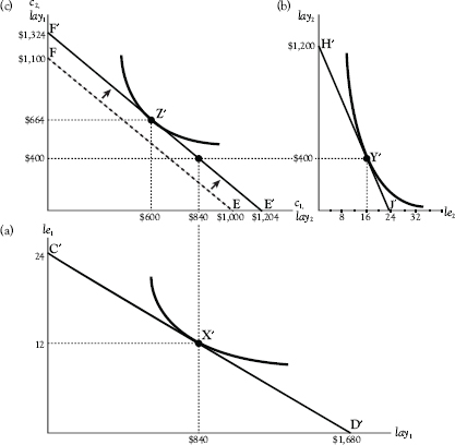
Figure 3.6 The two-period model with a change in wage rates

Adam decides to set his period-1 consumption at $600 and his period-2 consumption at $664.

We can take a policy lesson away from this demonstration. In the Keynesian model, to be examined in Volume II, Chapter 3, current consumption equals some fixed fraction of disposable income, and saving is the residual that is left over after spending. The role of government in determining consumption (and saving) derives from its power to raise or lower disposable income through the exercise of monetary and fiscal policy.

In this chapter, the individual decides what fraction of his income to allocate to consumption on the basis of the comparative utility of consumption now versus consumption later. The role of government is to determine how its policies affect this decision, given that its policies, in particular its tax policies, affect the reward for saving and therefore the funds that are available to finance capital spending. Our task, later, will be to consider which model better fits current economic circumstances.

Returning to our model, another possibility is that r would change. See Figure 3.7. There we replicate Figure 3.4, except that the interest rate rises to 15%. The effect of the higher interest rate is seen in the rotation of the budget line from FE to F′E′. Now, because the interest rate and, therefore the cost of borrowing, is higher, the individual finds that the maximum amount Adam can allocate to current consumption falls from $1,000 to $978. By the same token, the maximum amount he could allocate to future consumption rises from $1,100 to $1,125. In this example, period-1 consumption falls from $400 to $300, and period-2 consumption rises from $660 to $780.

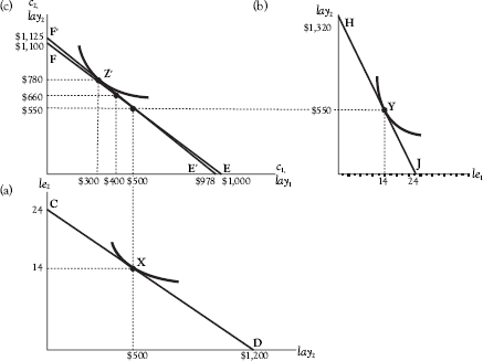
Figure 3.7 A rise in the interest rate in the two-period model

The Work-Now/Work-Later Choice

Next consider how Adam’s work-leisure calculus would take into account not just the wage rate he gets now but also the return on his saving and the wage rate he might get in the future. It is intuitively clear that a high return to current saving will induce people to work more now. If Adam believes that the stock market will head straight up for the next few years but may not thereafter, he would have reason to work hard now so that he can save now and enjoy the fruits of his efforts later when the market goes down. Likewise, if Adam realizes that he is in his prime earning years, he will want to work hard now in order to save up for the years to come when his earning power will be diminished. Think about athletes who figure that they have until age 40 to make the big money and scientific geniuses who are convinced that they must make their score before they turn 30, after which their mental capacities will never again be so keen. This is as opposed to piano soloists and some college professors who keep going until they drop.

To simplify the problem, let’s suppose Adam figures that he can make $50 an hour today but $25 an hour a year from now. Put differently, the cost of leisure for him now is twice what it will be in a year. Adam has an incentive to work especially long hours now, given that the reward for working will fall by 50% next year.

Suppose further that Adam can get 10% interest on a CD that will mature in one year. If he puts the $50 he makes by working an additional hour into the purchase of that CD, he will have $55 to spend next year. Now fast forward to next year, when he collects that $55 on the matured CD. With that much money, he can “buy” himself 2.2 (= $55/$25) hours of leisure: He does this by using the CD to replace the income he would lose by reducing his work time by 2.2 hours.

This tells us that the sacrifice entailed by taking another hour of leisure now can be seen in either of two ways: First, and as we have already seen, it entails the sacrifice of current income and therefore current and/or future consumption. Second, and alternatively, it entails the sacrifice of future leisure. The cost to Adam of another hour of leisure now is the 2.2 hours of leisure that he would have to sacrifice next year because of the labor and asset income that he sacrifices by taking that hour of leisure now. We can also say that if he gives up an hour of leisure today, he could reward himself with 2.2 more hours next year. Would it be in Adam’s interest to give up that hour of leisure now? As usual, we need to do some math to tackle this issue.

Let the marginal rate of substitution of current for future leisure (MRS_Le1Le2) be the amount of leisure Adam would give up in period 2 for another hour in period 1. Let’s refer to period-1 leisure as current leisure and period-2 leisure as future leisure. In this example, he has to give up 2.2 hours of future leisure for another hour of current leisure. Suppose (1) that the MRS_Le1Le2 = 2.5, meaning that he would be willing to give up 2.5 hours of future leisure for another hour of current leisure. Because it costs only 2.2 hours of future leisure to have another hour of current leisure, he will want to expand current leisure and contract future leisure.

Now suppose (2) that Adam’s MRS_Le1Le2 is 1.5, so that he is willing to give up only 1.5 hours of future leisure for another hour of current leisure, whereas it costs him 2.2 hours of future leisure for another hour of current leisure. In that instance, he would have expanded his period-1 leisure too far and would want to contract current leisure and expand future leisure.

Only when the amount of future leisure that Adam is willing to sacrifice for another hour of current leisure just equals the amount of future leisure that he must sacrifice for that additional hour of current leisure has he adjusted his work-leisure choices for both periods optimally. Formally, we write that Adam should adjust those choices so that

The cost of another hour of current leisure is which is to say, the amount of future leisure Adam must sacrifice in order to have that additional hour of current leisure. Adam will want to adjust his choices of leisure in both periods in such a way as to bring the value he places on current leisure, as measured by the value of MRS_Le1Le2, into line with this cost.

Let’s think about what this means to the macroeconomy. Suppose, in the forgoing example, that Adam has adjusted his allocation of leisure time between the two periods in such a way that he has satisfied equation (2.29):

Now suddenly Adam’s period-1 wage rate rises from $50 to $90.91 while his period-2 wage rate and his MRS_Le1Le2 remain unchanged. Temporarily now

the price of current leisure has risen from 2.2 to 4 hours of future leisure. Adam has an incentive to contract current leisure and expand future leisure. That is to say, he would want to expand current work and contract future work.

Alternatively, suppose that r rose from 10 to 15%, while the wage rate and his MRS_Le1Le2 remain unchanged. Here again, the cost of current leisure would rise. Now he would face the following situation:

Here again, there is an incentive to contract current leisure and expand current work, inasmuch as the cost of an hour of current leisure has risen from 2.2 to 2.3 hours of future leisure.

In this process, we encounter another version of the familiar idea of diminishing marginal rate of substitution. If Adam is in equilibrium to begin with and falls, he will want to bring his MRS_Le1Le2 back into line with by expanding current leisure and contracting future leisure, through which process his MRS_Le1Le2 will fall until it equals

On the other hand, if, and as in the forgoing examples, he is in equilibrium to begin with and rises, he will want to substitute future leisure for current leisure until his MRS_Le1Le2 rises to equal

The analysis so far provides some hints about the effects of government policy changes on individual behavior. We have seen, for example, that, acting rationally, people have an incentive to spread the effects of changes in current income over their future and present consumption. We will see that this is important in thinking through such matters as the burden of government debt on future generations and the effects of government policy changes on asset income.

Also, insofar as government can influence the wages that a person earns, policies that have the effect of increasing take-home pay (i.e., wages minus income and payroll taxes) can induce people to work more, just as policies that reduce take-home pay can induce them to work less. Our examples in Figures 3.4 and 3.6 showed as much, anyway. Finally, policies that cause a rise in the return to financial assets can induce people to work more and to save more.

It turns out, however, that things are not so simple. To see why, we have to recognize the distinction between substitution and income effects.

Substitution Versus Income Effects

Let’s consider the scenario illustrated by Figure 3.8. Adam is initially at point X on line AB, where he receives a wage of $50 per hour and chooses 14 hours of leisure (hence, 10 hours of work) and $500 in labor income. Then his boss raises his wage from $50 to $100 per hour, putting Adam on line BC, where he chooses to work 12 hours and earn $1,200.

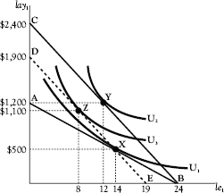
Figure 3.8 Separating substitution and income effects

We need to see how this rise in the wage rate exerts a substitution effect and an income effect on Adam’s leisure-income choice. Before the wage rate rose, the opportunity cost to Adam of each additional hour of leisure was $50. Because that cost has now risen to $100, Adam will have an incentive to substitute work for leisure. The substitution effect occurs as a result of this change in the opportunity cost of leisure. The individual will always expand work at the expense of leisure when his wage rate rises, if we ignore the fact that the higher wage rate also makes him richer. But because it does make him richer, it also exerts an income effect that works in just the opposite way of the substitution effect.

In Figure 3.8, we see how it is possible to separate these two effects. Recall that Adam, hard worker that he is, decided to increase his work day from 10 to 12 hours, that is, to reduce his leisure from 14 to 12 hours. This takes him from point X to point Y. Now an economist comes along and suggests an experiment to Adam’s boss. Under the experiment, his boss will tell Adam that the higher wage is still available but only if Adam agrees to contribute $500 a day to the boss’s favorite charity. This puts Adam on line DE. Now Adam finds that if he were to return to point X and continue working the same 10 hours that he did before his wage was increased, his take-home pay would be only as high as it was before, which is to say, $500. By working 10 hours, he would earn $1,000 but, by being forced to give away $500 of that amount, he would be back to bringing home only $500.

However, Adam will not return to point X. Because the opportunity cost of leisure has risen and because he is now $500 poorer than he would have been had he not been forced to give away $500, he would shift to some point on DE such as Z, where he would work something more than 10 hours a day. In this example, he decides to work 16 hours a day (reducing his leisure to eight hours a day) and makes $1,600 before having to pay the $500 to the charity, leaving him with $1,100 in take-home pay.

Eventually, in this scenario, the experiment ends. Adam’s boss says that Adam no longer has to give up $500 of his earnings and Adam is allowed to return to point Y, where he lives happily ever after. The purpose of this experiment was to isolate the substitution effect from the income effect of the wage change. The substitution effect was the adjustment from X to Z and the income effect was the adjustment from Z to Y. Stripped of the income effect, Adam expands his work by six hours. With the income effect, he expands it by only two hours. The reason why the income effect causes him to reallocate two of those hours back to leisure is that leisure is desirable and becomes more affordable at a higher wage.

This demonstration reminds us that as wage rates rise, we should expect the quality of life to rise, not just because higher wage rates increase people’s spending power but also because they permit people to allocate more time to leisure. Even if the individual ends up working more, as here, he has the option of working less while maintaining his standard of living.

Let’s see how a rise in the wage rate affects the supply of labor. Figure 3.9 traces the effects of the preceding experiment on Adam’s supply of labor. When the wage rate is $50, Adam is at point A and supplies 10 units of a labor. When the wage rate rises to $100, he increases his supply of labor to 12 (point B) or 16 (point C) units depending on whether the income effect is present or not. Figure 3.9 shows that there are two labor supply curves along which Adam could adjust—one that includes the income effect and one that includes only the substitution effect.

The alert reader will see that, if the income effect were large enough, Adam could actually reduce the quantity of labor he offers to his employer when his wage goes up. Yes, the substitution effect would induce him to provide more labor, but if the income effect is large enough it might overwhelm the substitution effect and he might, in the end, supply less labor.

This possibility comes up in discussions about tax policy. We will delve more deeply into tax policy in a later chapter, but we can see the outline of the problem now. “Supply-side” economists argue that if government taxes labor income at a lower rate, people will work more because their after-tax wage will rise and when they work more, the economy will expand as more labor enters production. But what if the income effect dominates and people respond to the increase in their take-home pay by working less rather than more?

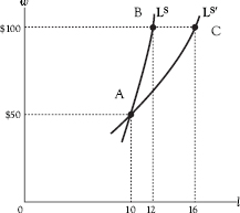
Figure 3.9 Labor supply with and without the income effect

One answer is that it shouldn’t matter how they respond. A rise in take-home pay is welfare-enhancing whether the person whose pay rises enjoys benefits in the form of increased pay or increased leisure. Much of human progress is measured by the opportunities for leisure and the reduced onerousness of work that has come with technical progress and capital accumulation.

Income effects are also present when there is a rise in the return to saving (r in our examples). We go into this matter in much greater depth in the next chapter. But for now, look back at Figure 3.7, where we let an increase in r bring about a rise in saving. That same increase in r could, however, have also led to a decrease in saving as Adam took advantage of the higher r to increase current consumption. An increase in r increases the cost of current leisure but it also makes current consumption more affordable. We begin the next chapter with a consideration of the income effect of a change in r.

Policy Implications

While some might see these distinctions as nuances, they, in fact, have great importance in forging macroeconomic policy. A principal goal of macroeconomic policy is to increase work and saving (even though leisure and present consumption are good things, too). This goal derives its appeal from the fact that production is good and that it occurs because of the application of labor and capital to production. In order to get more production, some combination of the following must occur:

These are the timeless and everywhere-applicable conditions for increased production. This chapter had to do with items 1 and 2. Insofar as people want to save more as the return to saving rises and insofar as workers want to work more as wage rates rise and insofar as government can affect these variables, we see an opportunity for government to expand output.

This chapter was about the individual choices that drive the decision to supply labor and to save. For all the minutiae through which we had to wade, we covered only half the story on the matter of saving and work. The other half of the story concerns what must be true so that investors will want to apply saving to capital formation and so that employers will want to hire the labor supplied to them.

So what have we learned so far? Actually, two important things. First, increases in wage rates will increase the amount of labor people will want to supply, provided any income effect exerted along the way is less than the substitution effect. Second, increases in the return to saving increase saving provided, again, that any income effect is less than the substitution effect. Thus if the goal is to increase the supply of labor and to increase saving and if conditions are suitable, then government should adopt policies that cancel out the income effect. We will consider just what sorts of policies might do that in Volume II.

Also important in later chapters is the question of how workers respond to changes in what we can call the “net real wage rate.” This is the inflation-adjusted wage that the worker receives after accounting for any reduction in his inflation-adjusted real wage that results from his incurring an additional tax liability or from his sacrificing a government benefit by earning another dollar of labor income.

Suppose that Adam’s boss pays him a gross wage of $50 for an hour’s work. (We will ignore how inflation affects Adam’s real wage for the purpose of this example.) Suppose further that either (1) Adam has to pay 25% of his wage in income tax or (2) he has to forego 25% of his wage under a means-tested welfare program from which he receives benefits. In either event, his net wage is $37.50 (= 0.75 × $50). It is to changes in this net wage that Adam will respond in adjusting his work-leisure calculus.

An important question for purposes of considering the efficiency (or “classical”) effects of policy changes is how workers respond to changes in their net wage. The more they respond, the greater the amount of labor that will be supplied to producers for any increase in the net wage brought about changes in tax rates or benefit formulas.

One measure of this responsiveness is the Frisch elasticity of labor supply. As described by economist Casey Mulligan, whose work we will examine closely in Volume II, the Frisch elasticity

Mulligan considers Frisch elasticities between 0.4 and 1.1 (Mulligan 2012). The authors of another study report that the Congressional Budget Office uses Frisch elasticities that range from 0.27 to 0.53, with a central estimate of 0.40 (Reichling and Whalen 2012, p. 3). These elasticities become important when considering how reductions in tax rates or social benefits affect labor supply.

¹ A clarification about signs: In calculating the MRS_LeLay, we assume either that labor income rises as leisure falls or that labor income falls as leisure rises. Thus must be negative. Because we want to think of MRS_LeLay as a positive number, we thus place a minus sign in front of to get MRS_LeLay. We follow this convention throughout the book.

² Absolute value means numerical value. The slope of a downward sloping line is negative, but it is more convenient to speak in terms of the numerical value (say, 100) of the slope, rather than the actual value of the slope (say, –100). To make the language less cumbersome, we will often talk about the “slope” of an indifference curve even though we really mean the absolute or numerical value of the slope.