CHAPTER 4

Saving

In Chapter 3 we saw that the return to saving r enters into the decision whether to consume or save. There we alluded to the fact that the effect on saving of a rise in the return to saving depends on the relative strength of the substitution and income effects at work.

The substitution effect results from the fact that, with a higher r, the individual finds that each dollar added to saving brings a higher return in the form of increased future consumption than it did before. If r rises from 5 to 6%, the individual gets $1.06 to apply to next year’s consumption for every dollar saved, rather than $1.05. This operates to increase saving. A rise in r can be thought of a rise in the price of current consumption, as measured by the amount of future consumption foregone for each dollar allocated to current consumption.

The income effect results from the fact that an increase in r makes it possible to increase current consumption, and therefore reduce current saving, without reducing future consumption. Suppose that when r = 5% the individual saves $10,000. By saving $10,000 this year, he will have $10,500 more to spend next year. If r rises to 6%, he could reduce his saving to $9,906 (= $10,500/1.06) this year and still have $10,500 more to spend next year, given the rise in r. (For the time being, ignore the fact that this rise in r would reduce the present value of his income.) This creates an income effect equal to the difference between $10,000 and $9,906, which is the $94 by which he could reduce his current saving and increase his current consumption without suffering any loss in future consumption.

If, in this example, the rise in r induces the individual to increase current consumption and therefore decrease current saving, we say that the income effect more than offsets the substitution effect. If it induces him to decrease current consumption and therefore increase current saving, then the substitution effect more than offsets the income effect. If it induces him to keep his current consumption and saving constant, then the two effects exactly offset each other. Thus, under this last possibility and in the current example, the individual would have $10,600 to spend next year, which is exactly 1 percentage point more (the difference between 5 and 6%) than what was available to spend before the interest rate rose by 1 percentage point.

Alternative Views of Saving

A question of central importance to economic policy is whether a rise in the return to saving, as brought about by a reduction in the taxes on the return to saving, will cause saving to rise and by how much. The relative strength of the income and substitution effects is one factor to be considered while addressing this question.

There is another factor to be considered, which has to do with how saving responds to changes in income, given that there is no change in r. The long-run, classical view is that the individual simultaneously chooses his level of work effort and saving toward optimizing his lifetime utility. In this view, any unexpected change in current income manifests itself in a change in planned consumption over the individual’s future. If the individual unexpectedly sees an increase in current income, he will allocate only a small portion of that increase to current consumption, saving the remaining portion to finance future consumption.

In the short run, however, when there is low-employment equilibrium, brought about by either excess aggregate supply or excess aggregate demand, things are different. Individuals cannot optimize their consumption–saving choices because they cannot optimize their work–leisure choices. In a Keynesian slump, employers will not use all the labor services workers want to provide. In a suppressed inflation slump, workers will not provide all the labor services employers want to hire. In both instances, workers’ current income and current consumption are constrained by an imbalance between aggregate supply and demand. Government policies that are effective at correcting that imbalance will manifest themselves mainly in increases in current consumption.

This presents an empirical question: Do government correctives for a perceived imbalance between aggregate supply and aggregate demand result mainly in an increase in current consumption or saving? If they result in more consumption, then the diagnosis and the corrective can be deemed successful. If they result in more saving, then the diagnosis was wrong and the policy was wrongly applied. We consider some modern evidence bearing on this matter in Volume II.

Going Back to the Classical Model

Proceeding in the spirit of the classical model, there are two central questions: (1) How do changes in the return to saving r affect saving and (2) how much of an effect on current consumption (and therefore current saving) do changes in current income have? Let’s address the first question first.

In Chapter 3, we assumed the existence of a saver named Adam. In the interest of gender equity and of adding some variety to the exposition, let’s switch decision makers from Adam to Eve, and let’s imagine that the young Eve, now out of the Garden of Eden, is about to begin a career over which she expects her income to follow a predictable pattern, rising from year to year until retirement.

Eve understands that each year, her saving or borrowing decision affects her future income and therefore her future consumption. She understands that her earning power will max out only as she approaches retirement and then, as we assume here, drop to zero. But she also realizes that she has the option, when she is young, of spending either less than she earns (in which case she saves) or more than she earns (in which case she borrows). If she wants to save for a comfortable retirement, she can save when she is young so that she can spend more later. On the other hand, if she is in a hurry to spend when she is young, she can borrow (to a degree at least) against her future income to finance current consumption. Later we will consider the possibility that she would want to borrow when young, save when middle age, and then dissave when old. But the general idea is that Eve is not constrained to spend only (or all) her current income.

The reality, of course, is that Eve’s expectations about her future income can change moment to moment, as can the return to her saving r. In this chapter, we think of r as “the” interest rate, the rate at which Eve can alternately lend or borrow money. To simplify our thinking about Eve’s thinking, we can imagine that every January 1, she reassesses her income prospects and makes a forecast of r for the purpose of planning her consumption and therefore her saving for the year to come and that she does this every year going forward all the way to the end of her planning horizon.

In performing this annual recalculation, Eve recognizes r as serving two roles: For one thing it measures the return to saving and, likewise, the cost of borrowing. For another, it serves as the discount rate for calculating the present value of her future income. The higher the r, the greater the return to saving, the greater the cost of borrowing, and the lower the present value of future income. If Eve wants to use $1,000 of her income next year to buy a TV now, she can borrow $952.38 (= $1,000/1.05) now to apply to that purchase if r equals 5%, but only $909.09 if r equals 10%.

We presented this present-value accounting in Chapter 3 in our discussion of Adam’s choice calculus. But there we posited Adam as being a saver. A better theory would account for the possibility that he or Eve could switch from being a saver to a borrower or vice versa. So how will a change in r affect the decision to save or borrow?

The question of how changes in r affect Eve’s lending or borrowing depends on how r enters into her consumption–saving decision. (Remember that lending is positive saving and borrowing is negative saving or dis-saving.) We will shortly go into some detail figuring out how the rational Eve would decide between consumption and saving, given whatever r she faces in the market for loanable funds.

Now let’s turn to a second question. Suppose Eve hits the lottery and brings home a check for a million dollars. (We will ignore taxes and the fact that the actual immediate payoff from a lottery is always much less than the advertised payoff). Unless Eve is foolish, she will not blow through the entire million dollars on the spot. Rather, she will spread out the benefits of her prize over her future, which will be very long if she is very young. She might even care about her future children and their future children. So the question is how much of her prize will Eve spend when she cashes the check. This is part of the general question whether a surge in current income will have much of an effect on current consumption.

Expanding the Saver’s Time Horizon

Recall that in our two-period model, we calculate saving in period 1 as

We now allow that Eve plans her consumption and saving over as long a period of time as she wishes to consider. We treat this period as beginning with year 1 and ending with year n. We allow that Eve can save or dissave (which is to say, borrow) as much as she wishes during any year t = 1, 2,…, n – 1, given that she will consume all she can in period n. We also allow that she receives a combination of labor and capital income over the course of her lifetime. So her total y_t in any period t is

where nw_t is capital or asset income.

Now

Note that Eve’s saving rate can be positive, negative, or zero: positive if she consumes less than she earns in income, in which event she uses part of her income to augment her asset holdings, zero if she consumes all of her income, and negative if she supplements her consumption by drawing down her asset holdings.¹ This definition of the saving rate is useful because it corresponds to the common-sense idea that peoples’ saving rate will be negative when they are young or old, and likely to spend more than they earn, and positive when they are middle-aged, and likely to spend less than they earn, to pay off debts incurred when young to acquire assets to spend down when old.

Now let’s construct a specific utility function, which shows how many utiles Eve gets from consumption in any one period. A utility function that macroeconomists frequently use for this purpose is as follows:

While this specification may look complicated, the reason that it is so popular is similar to the reason (as we shall see) that the Cobb-Douglas specification of the production function is so popular, namely, that it is easy to work with. We will shortly see why this is true. For now, the only thing that’s new is the parameter z. The name of the reciprocal of is the intertemporal elasticity of substitution (IES), which measures the sensitivity of Eve’s consumption (and therefore saving) decisions to differences between the return to saving r and her rate of time preference ρ, as considered in Chapter 3.

We have already seen that when an individual maximizes utility, he (or in this instance, she) satisfies the following equation for a two-period model where t is period 1 and t + 1 is period 2:

the left-hand side of which can be expanded to read:

Generalizing the two-period model to n periods and substituting equation (4.6) into equation (4.7), Eve maximizes utility when

Now let’s use an example to flesh out equation (4.8). Suppose that Eve’s planned consumption is $50,000 in period t and $55,000 in period t + 1, and let z equal 0.5. A $1 change in her consumption in period t will cause her utility to change by

Correspondingly, a $1 change in her consumption in period t + 1 will cause her utility to change by

Finally, assume that Eve’s rate of time preference r equals 5%, so that

Plugging the information from equations (4.9), (4.10), and (4.11) into the left-hand side of equation (4.8), we get

Then also from equation (4.7),

Equations (4.9) and (4.10) tell us that an additional dollar of period t consumption adds as much to Eve’s period t utility as an additional $1.0465 (= 0.0045/0.0043) of period t + 1 consumption adds to her period t + 1 utility. If Eve gives up $1.00 of consumption in period t + 1, she loses 0.0043 utiles in period t + 1, but if she adds $1.00 dollar to her consumption in period t, she gains 0.0045 utiles in period t. So she can give up as much as $1.0465 of her period t + 1 consumption while increasing her period t consumption by $1 and at the same time keep the sum of her utilities over the two periods constant. But because a period-t utile is worth 5% more than a period t + 1 utile, she is willing to give up $1.10 (= 1.0465 × 1.05) of period t + 1 consumption for another dollar of period t consumption. If r equals 10%, she satisfies the equilibrium condition of equation (4.6).

Maximizing Intertemporal Utility

Now we get to find out why the specification of Eve’s utility function in equation (4.5) is so popular. It turns out that, after a lot of mathematics using equation (4.5), as shown in the Appendix to this chapter, we can transform equation (4.6) into the following equation:

This tells us that when Eve is maximizing utility, the percentage change in her consumption from one period to the next equals the difference between r and ρ multiplied by which we previously identified as Eve’s intertemporal elasticity of substitution (IES). We can simplify even more by rewriting equation (4.14) as

We can also now see exactly what IES means. The IES is the number of percentage points by which the desired consumption in the next period will exceed consumption in the current period for every percentage point by which r exceeds ρ. (Or, if r exceeds ρ, the number of percentage points by which desired consumption in the next period will fall below consumption in the current period for every percentage point by which r exceeds ρ.)

Before thinking more about what this equation says, let’s see if Eve maximizes her utility by increasing her consumption from $50,000 to $55,000 going from period t to period t + 1. Her planned percentage change in consumption (%Δc) is 10% (= $5,000/$50,000). The question is whether this planned percentage change in consumption will maximize her utility. According to equation (4.15), it does if (r − ρ)IES also equals 10%. Well, let’s see if it does: First, (r – ρ) equals (10% – 5%) or 5%. Next, because z equals 0.5, 1/z, which is the IES for Eve, equals 2. Thus, we have 0.05 × 2 or 10%. Eve does, in fact, maximize her utility!

The utility function specified in equation (4.5) thus turns out to have a convenient property, which lies in the fact that the coefficient 1/z measures the sensitivity of the individual’s consumption plan to the difference between r and ρ, which is to say, to the difference between the return to saving and the individual’s time preference.

As we know, r and ρ can change from moment to moment, but there is little sacrifice in generality if we continue to think of Eve as revising her plans for her economic future every January 1. The questions for this chapter are (1) what will be her year-1 consumption and saving and (2) how would a change in r or in her current and future income affect her year-1 consumption.

According to the usual view of Eve’s saving decision, she would put aside some fraction s of her disposable income each year based on some combination of future needs (the wish to own her own home, the education of her kids, her retirement, etc.). This is all right as far as it goes, but the rational Eve understands that the money she has available to apply to her saving now will affect her consumption in every year of her life going forward (just as her income in every year of her life going forward affects her ability to consume and save). So the rational Eve needs to put together some information in order to decide how much to consume and save in every year of her life starting now and going forward. Specifically, she needs to know:

Knowing this, she can figure out how much of her income to allocate to her current-year consumption and therefore her current-year saving. Once she knows that, she can apply equation (4.15) to figure out her second-year consumption, and then again to figure out her third-year consumption, and so forth. (Keep in mind that her second-year consumption will equal her first-year consumption times (1 + %Δc), where %Δc is determined once she knows what values to assign to r, ρ, and IES.).

Again, understand that economists don’t require Eve consciously to make all these calculations. The computer she carries around in her brain can do all that without her explicitly thinking about it. Yet, as strange as this might seem to the noneconomist, everything here is based on common sense. One way or another, Eve’s consumption in 2019 will bear some relationship to her consumption in 2018. The greater the reward to saving (r), the less impatient she is for current consumption (the lower her ρ), and the more she wants to substitute future for current consumption, given the difference between r and p, the more she will want her next-period consumption to exceed her current-period consumption. And then also, the more she will want to save in the current period.

Suppose the computer in Eve’s head has already solved equation (4.15) on January 1, 2018, and then, seconds after midnight, she finds out that r has unexpectedly risen. Because this raises the return to saving and the cost of borrowing, Eve will want to rethink her spending plans for the year to come and for every year thereafter. Because her spending plans and her saving plans are just opposite sides of the same coin, she will likewise want to rethink her saving plans.

The same would happen if her rate of time preference ρ or her IES changed. Then once Eve has adjusted the left-hand side of equation (4.15) accordingly she will be back in utility-maximizing equilibrium. But Eve needs to figure out her year-1 consumption and saving before she can figure out how much more (or less) to spend on consumption in year 2. Equation (4.15) just tells us the percentage by which she will want to change her consumption going from the current period to the next. Let’s identify the current period as year 1. Then Eve still needs to figure out how much to consume in year 1, after which she can plot her consumption plans all the way to retirement.

Last Step

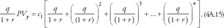
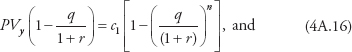
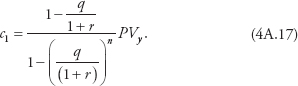
To figure out Eve’s year-1 consumption, we need to reintroduce an assumption from Chapter 3, whereby Eve will set the present value of her current and future consumption in year 1 equal to the present value of her current and future income. Let’s write that condition as

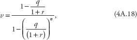
Given that assumption and equation (4.5), we can find a coefficient v, which when multiplied by the present value of Eve’s income will tell us how much she wants to consume in year 1. Generally, Eve’s period-1 consumption is

her period-1 saving is

and her saving rate is

The Appendix to this chapter shows how to calculate v. In general:

Point 1 means that saving will be greater the higher the r and higher the IES. Point 2 means that changes in r will not affect the fraction of PV_y that is allocated to saving when IES =1. This goes to the relative strength of the income and substitution effects. The income and substitution effects must just offset each other when IES = 1. To see why, recall the example with which this chapter began. There we saw that a 1-percentage-point rise in r this year would bring about a 1% rise in the funds available for consumption next year without the need to increase saving. The same applies here, but more generally: If r is constant and IES = 1, the percentage change in consumption from one year to the next will rise for every percentage point increase in r but without an increase in saving.

The reader may well (and should) question the validity of equation (4.16), given that the present value of lifetime consumption for some people will far exceed the present value of their income. Those people include people who are lucky enough to be born rich and some others who sustain themselves from government transfer payments. Given that 72% of disposable personal income comes from wages, this, sadly perhaps, is not a widespread problem. And even trust-fund babies can come to see the value of work as they look to pass along their legacy to their progeny.

How Changes in r Affect Saving

Whether saving does or does not rise in year 1, given a rise in r, also depends on how a rise in r affects the present value of income. Remember that year-1 consumption equals v times the present value of income and that year-1 saving equals year-1 income minus year-1 consumption. Because a rise in r will reduce the present value of future income, a rise in r will for that reason alone reduce current consumption and therefore increase current saving.

To put some numbers to this analysis, suppose that IES = 1 and that we are back to a two-period world. Then we know that Eve’s desired percentage change in consumption from period 1 to period 2 will rise by one percentage point for every percentage point that r rises, ρ remaining constant. Now let’s make some more assumptions:

From the Appendix we can use this information to find v, which turns out to be 50.495%. (The shorter the individual’s time horizon, the larger v.) Table 4.1 shows the results for period-1 saving and for periods 1 and 2 consumption.

Now let the interest rate rise to 6% while all the other assumptions remain unchanged. Table 4.2 provides the results.

We see that saving rose, but not because v fell. Saving rose entirely because the present value of income fell. When IES = 1, a rise in the interest rate therefore does not affect current consumption or current saving, except insofar as it reduces the present value of income.

A rise in r will induce Eve to increase her saving rate because it will reduce PV_y and therefore current consumption. Conversely, a fall in r will induce Eve to decrease her saving rate because it will increase PV_y and therefore current consumption. It is just that her saving rate will change more, the larger her IES.

Table 4.1 Two-period model (r = 5%)

PVy	$100,000a
c1	$50,495b
sav1	$9,505c
s1	15.84%d
sav1(1 + r)	9,980e
c2	$51,980f
Δc/c	2.94% g

a = $60,000 + $42,000/(1.05); b = 0.50495 × $100,000; c = $60,000 – $50,495;
d = $9,505/$60,000; e = $9,505 × (1 + 0.05); f = $42,000 + $9,980;
g = ($51,980 – $50,495)/$50,495

Table 4.2 Two-period model (r = 6%)

PVy	$99,623a
c1	$50,305b
sav1	$9,695c
s1	16.2%d
sav1(1 + r)	10,277e
c2	$52,277f
Δc/c	3.92%g

a = $60,000 + $42,000/(1.06); b = 0.50495 × $99,263; c = $60,000 – $50,305; d = $9,695/$60,000; e = $9,695 × (1 + 0.06); f = $42,000 + $10,277; g = ($52,277 – $50,305)/$50,305

Suppose that IES equals 1.5. Eve will want the percentage change in her consumption to equal 1.5 percentage points for every percentage point rise in r (again, holding ρ constant). The substitution effect of the rise in r will more than offset the income effect.

Let’s make our analysis more realistic now by assuming that Eve takes her first job on her 22nd birthday and that the job offers a starting salary of $50,000. Eve expects to retire in 40 years, when she is 62, and expects to get a 5% raise each year she is on the job (which means she’ll make about $335,000 dollars the last year she works!). We assume that, for convenience, the interest rate is initially also 5%. Finally, we assume that Eve has a rate of time preference of 2% and an IES of 1.5.

Discounted over Eve’s 40-year working life, the present value of her income is $2,000,000. Given our assumptions, Eve’s v is 2.77%, and her first-year consumption is $55,400 (see footnote a to Table 4.3). She plans that, during the first year of her career, her saving will be a negative $5,400 and her saving rate will therefore be –10.8%. Her planned year-2 consumption is $57,893, which, given the values assigned to r, ρ, and IES must be 4.5% greater than her year-1 consumption.

Now suppose that, just after Eve had planned out her current and future consumption, the interest rate rose unexpectedly to 6%. Eve’s income stream remains unchanged, but her v falls to 2.53%.

The present value of her income stream falls to $1,672,452. Thus, she revises her plans so that she will consume $42,313 in the first year and $44,852 in the second. She will increase her first-year saving from –$5,400 to $7,687 and her saving rate from –10.8 to 15.4%.

We can infer that a given rise in the return to saving produces a larger rise in Eve’s saving rate as her IES exceeds 1. But whatever the value of her IES, v will always be small when the planning period extends well out to the future. To see this, let’s consider a few more examples. In Table 4.4 we assume that ρ = 0.02, n = 40, r = 0.05, and lay₁ = $50,000. The larger Eve’s IES, the smaller her v and the larger her s.

Table 4.3 Lifetime model: Effects of a rise in r

	r	v	PV1	c1	c2	sav1	s1
Initial values	5%	2.77%	$2,000,000	$55,400a	$57,893b	–$5,400c	–10.8%d
Values after r rises	6%	2.53%	$1,672,452	$42,313e	$44,852f	$7,687g	15.4%h

a = 0.0277 × $2,000,000; b = $55,400 × (1 + ((5% – 2%) × 1.5)); c = $50,000 – $55,400; d = –$5,400/$50,000; e = 0.0253 × $1,672,452; f = $42,313 × (1 + ((6% – 2%) × 1.5)); g = $50,000 – $42,313; h = $7,687/$50,000

Table 4.4 Effects of IES on the saving rate

IES	v	s1
0.1	5.34%	–113%
0.5	4.52%	–81%
1.0	3.58%	–43%
2.0	2.08%	17%
2.5	1.52%	39%

Assume again that Eve’s first-year income is $50,000 and that she has a v = 2.77%. Now she hits the lottery and brings home $1,000,000. Eve’s PV_y rises from $2,000,000 to $3,000,000. Given her v, her consumption will rise from $55,400 to $83,100. After winning $1,000,000 she will increase her current-year consumption by only $27,700! This dampens any hope of economic recovery through a fiscal stimulus, a matter to which we will return in Volume II.

As shown in the Appendix, these calculations are greatly simplified if we assume that IES = 1 and n is large. Then

If, under these conditions, ρ = 2%, a million-dollar bonus in year 1 will increase consumption in that year, and in every year to follow, by $19,608.

The Permanent Income Hypothesis

These observations are consistent with the permanent income hypothesis, which states that people make spending decisions according to how a change in current-period income affects their permanent income. We see that if the rational Eve experiences a change in her current income (even a change of $1 million) she will adjust her current consumption according to how that change affects the present value of her current and future income and according to the size of v. And if Eve has a long planning horizon even large changes in her current income will have small effects on this PV_y. So what is her “permanent income?”

One idea that motivates the concept of permanent income is that people will want to smooth out their consumption stream over their lifetimes to whatever degree is possible. The foregoing discussion provides examples in which the individual will have a consumption schedule that slopes steeply upward or steeply downward over her lifetime, depending on the size of r, ρ, and the IES. A high r and a low ρ indicate high saving at the beginning of the planning period but high consumption at the end. Just the opposite is true for a low r and a high ρ.

This means that actual income will vary from year to year, depending on a great many factors (including such things as lottery winnings), while consumption will follow some more or less steady path, depending on how the individual wants to structure his or her consumption over the planning period. Think of permanent income, then, as the individual’s consumption stream, however arranged, over his future. Hitting the lottery will always have a much smaller effect on permanent income than on current income since the lucky winner will want to spread his winnings out more or less evenly over her future.

There is an argument to the effect that permanent income, so defined, will be flat over that future even as actual current income rises and falls. Let’s see why the individual would not want to have a steeply rising or steeply falling consumption curve over her future.

If Eve is a high saver at the beginning of her life, her consumption will steadily rise over the course of her lifetime and the marginal utility of consumption will steadily decline. Using the notation developed earlier, would be high relative to . It seems that she would want to move some of her consumption from her later years, when the utility she would lose by taking a dollar out of consumption is low, relative to her early years, when the utility she would gain by adding a dollar to consumption is high. If she were to do this, would fall and would rise until, in the limit, they were equal. But then, as we see from equation (4.8), ρ would then have to rise until it was equal to r.

Conversely, if Eve is a high borrower at the beginning of her life, her consumption will steadily fall over the course of her lifetime and the marginal utility of consumption will steadily rise. would be low relative to . It seems that she would want to move some of her consumption from her early years, when the utility she would lose by taking a dollar out of consumption is low, to her later years, when the utility she would gain by adding a dollar to consumption is high. If she were to do this, would rise and would fall until, in the limit, they were equal. This time ρ would have to fall until it was equal to r.

This logic argues for a saving strategy that brings the rate of time preference ρ into line with the interest rate r. Return to equation (4.15) and consider what it means if ρ = r. Mathematically, the individual sets %Δc equal to zero for all periods going forward and thus equalizes consumption from one year to the next over the entire planning period. What seems intuitively plausible is that Eve would want to even out her consumption over life as much as practical. Every entrant into the labor force can reasonably expect his or her earnings to be low at first, then rise, and then drop precipitously upon retirement.

Neither Adam nor Eve will, however, want to eat sardines when young and old but then gorge on filet mignon when middle aged. In the language of economics, the marginal utility of the individual’s income will be high when his earnings are low, that is when he is young and when he is old, and the marginal utility of his income will be low when his earnings are high, that is when he is middle aged. Insofar as he wants to equalize the marginal utility of consumption across his lifetime, he will dissave (borrow) when young, save when middle aged, and dissave (use up assets) when old. Operationally, in our planning model, this means adjusting ρ to be equal to r, so that consumption is equal across the individual’s planning period.

This in turn means that in order for aggregate saving to be positive, we need to have a lot of middle-aged income earners who are accumulating assets even as younger and retired individuals dissave. It also means that we need tax policies that encourage saving, a matter taken up in Chapter 7.

Figure 4.1 illustrates the results of this strategy for the example provided in the first row of Table 4.3, with the difference that ρ and r are both assumed to equal 5%. There Eve’s annual income rises from $50,000 in year 1 to $335,000 in year 40, after which it drops to zero. (We assume that Eve spends her golden years living with her children, who generously subsidize her consumption beyond her planning period to her death.) She fixes her annual consumption at $111,000 per year from year 1 to year 40.

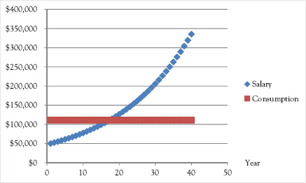
Figure 4.1 Illustration of permanent income hypothesis

Thus $111,000 per year is Eve’s permanent income. It is the consumption she would enjoy if she equalized her consumption over her lifetime, given her earnings expectations and the value of r. Eve’s permanent income is to be distinguished from her temporary income. If at some point in her life Eve wins $10,000 in the lottery, her temporary income will rise by $10,000, but her permanent income will hardly rise at all.

Eve would face myriad practical obstacles to a strategy that had her spending twice as much as she earns in her early years. There are practical obstacles to any consumption plan that requires borrowing against future income. In practice, young people dissave by taking out student loans, borrowing from relatives, and cashing in any inheritances they are lucky enough to receive. But a confident young Eve cannot go to her bank and take out a loan to buy a luxurious house, on the promise that she can pay off the loan without any problem in a decade or so. Liquidity constraints limit the practicality of any scheme requiring substantial borrowing against future earnings.

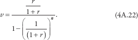
Yet the example is based on common sense and yields a handy tool for estimating the effect of an increase in current income on current consumption. As shown in the Appendix, v reduces to

if we assume that ρ = r and that n is large. Thus, if r equals 5% and if Eve wins $1,000,000 in the lottery, her spending in year 1 and in every year thereafter will rise by $47,619. This can be considered to be the classical analog of the marginal propensity to consume of the Keynesian model.

There is one overriding conclusion about the effects of windfall gains that can be taken from this chapter, which is that any such gain will yield a small increase in current consumption because of the desirability of “consumption smoothing,” which means spreading the benefits over the future rather than just taking them all at once. This bodes ill for government policies aimed at stimulating current consumption through tax rebates and the like.

In the aggregate, saving is positive. But if aggregate saving is positive year after year going forward then individual savers are regularly, and on balance, taking part of their income and putting it into income-earning assets on which they plan to draw in future years to finance their planned consumption. The existence of a positive national saving rate depends on the preponderance in the labor force of individuals who anticipate income decreases as they age and who want to accumulate income-earning assets during their peak earning years in order to pay off loans taken when young and to save for retirement.

Policy Implications

We shall see in Chapter 6 that a government policy that succeeds in raising the saving rate s can bring about an increase in real GDP per person. In Chapter 7, we will see how government can increase the rate of return to saving r and thus increase the individual’s saving rate by reducing taxes on capital income. The ability of government to increase s by increasing r depends, as we have seen, on the size of the IES. The greater the IES, the more effective are government policies aimed at increasing s. But is the IES large enough for those policies to be effective?

Economist Robert Hall has offered what is probably the most pessimistic assessment of the prospects for increasing the saving rate through the removal of tax deterrents to saving. As he puts it, his analyses provide “little basis for a conclusion that the behavior of aggregate consumption in the United States in the 20th century reveals an important positive value of the intertemporal elasticity of substitution” (Hall 1988, p. 356). See also (Braun and Jakajima 2012). Hall finds that increases in r have almost no effect (and might have a negative effect) on saving.

In contrast, Jonathan Gruber finds that the “estimated EIS [elasticity of intertemporal substitution, same as the IES] is very large, larger than most estimates from the previous literature, and this estimate is robust to a wide variety of specification checks” (Gruber 2013, p. 4). Gruber finds the value to be around 2 (Gruber 2013, p. 24). In his book The Redistribution Recession, Casey Mulligan puts the IES at 1.35 (Mulligan 2012, p. 152).

Perhaps, on the other hand, the size of the IES becomes less important when we consider the implications of the assumption, maintained throughout this chapter, that people base their current saving decisions on planned lifetime consumption. In this regard, David Romer considers the scenario in which “r is slightly larger than ρ and that the elasticity of substitution is small.” These assumptions “imply that consumption rises slowly over the individual’s lifetime. But with a long lifetime, this means that consumption is much larger at the end of the life than the beginning.” Then, given that income is constant,

This chapter delved into the saving calculus of the individual. In the next chapter we consider how saving decisions match up with capital investment decisions to determine investment and the equilibrium capital stock.

Appendix A

First we set the present value of utility equal to the individual’s consumption stream discounted by ρ:

Next we write out the formula for the present value of consumption:

We can write the individual’s utility maximization problem in terms of the Lagrangian expression:

Maximizing (4A.3) we get

for all t = 2,…, n.

and

where

Then

for all t = 1,…, n.

We can further simplify this by taking logarithms of both sides of (4A.8):

Now we set the present value of consumption equal to the present value of income:

Letting

we can write:

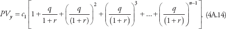
Then we can solve for c₁ by multiplying both sides of (4A.14) by and subtracting, to get

Solving,

If we let

then

c₁ = vPV_y.

Note that if the intertemporal elasticity of substitution, equals 1, q becomes and

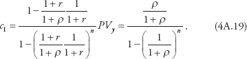
Then, as n approaches infinity, (4A.19) becomes

so that

We can also see that if r = ρ, then

Finally, in that case, as n approaches infinity,

¹ This is not the same as the conventional definition, according to which the saving rate equals personal saving divided by disposable personal income. Here there are no taxes, so disposable income equals personal income.

² This relies on a couple of mathematical tricks whereby we can approximate ln(1 + r) - ln(1 + ρ) as (r - p) and lnc_t - lnc_t-1 as