CHAPTER 7

Taxes and the Macroeconomy

Economists have a reputation for disagreeing among themselves, a state of affairs that some believe to disqualify them from commenting on anything. In fact, there are many propositions on which economists generally agree, if only implicitly. One is the law of diminishing returns. You cannot, as someone has pointed out, grow all the world’s wheat in a single flower pot. Presumably, also, no one would advocate raising the minimum wage to $100 an hour.¹

There is another proposition that can’t be doubted, and that is, at some point a further increase in the tax rate on whatever is being taxed will cause the government to bring in less revenue rather than more. The school dubbed “supply-side economics” has stressed this principle and correctly so. If the government taxed income at 100%, it would collect no revenue because either no one would bother to earn income or anyone who did would not report any income. This is not “voodoo economics,” as President George H. W. Bush called it, to his eternal discredit, but economics you can believe in (Romer and Romer 2010).

Of course, not even the most zealous progressive would advocate a $100 minimum wage or a 100% tax on income, but even less zealous progressives have to own up to an inconvenient (for them) truth, which is that as tax rates rise the base on which a tax is assessed (e.g., income) will ultimately shrink and that, as the tax rate approaches 100%, revenues will shrink to zero. Let t stand for the average tax rate on income. Then tax revenue (TR) in our version of NIPA accounting can be expressed as

This reminds us that in the real world of tax policy, the amount of tax revenue collected by government equals the tax rate applied to some tax base (here, income) and that the tax base itself depends on the rate at which it is taxed.

It takes only a little math to illustrate this point. Let Y (here, income or GDP) be the tax base, as measured to reflect the effect of t on Y, and let t be the rate at which income is taxed. We can then say that total tax revenue TR is simply the product of t and Y.

We can use this equation to compute the percentage change in revenue that results from a given percentage change in t as

To hear some progressives talk about tax policy, %ΔY is always zero or close to it. This is to say that if the tax rate goes up by 10% so will revenues. Thus government can make the tax rate as high as it wants without worrying that income, and eventually also tax revenues, will start to fall. When you hear people talk about “static” revenue estimates, this is what they mean. Such estimates presuppose a zero taxpayer response to any tax-law change. A given percentage increase in the tax rate always yields an equal percentage increase in revenues. That any policy maker or policy advisor would endorse such a principle is bewildering but true.

Static estimates belong in the same category as arguments about getting all the world’s wheat out of a single flower pot or raising the minimum wage to $100 an hour. Plausibly, when the tax rate is very low, a rise in the tax rate would have little effect on Y or might even, because of the income effect, cause Y to rise. But imagine that you are a worker making $50 an hour and already paying 75% of your hour wage in taxes, only to learn that now the government wants to collect 85%. Currently, the sacrifice of another hour of leisure lets you take home only an additional $12.50. Now the government wants you to take home only $7.50. At some point in this process you will surely discover that your time is better used in such untaxable pursuits as growing your own food or earning your income under the table.

If the government doesn’t want to collect any tax revenue on income, it just sets t to zero. But it is inevitable that as t rises, Y will at some point shrink, that is, %ΔY will become negative. Once Y starts to shrink, the effect of an increase in t on REV depends on how much %ΔY offsets %Δt. At some point, that sensitivity will be so high that further increases in t will cause revenues to fall, that is, the numerical value of %ΔY will exceed that of %Δt.

The Laffer Curve

This leads us to the famous Laffer curve, which, by legend, economist Arthur Laffer drew on a cocktail napkin for Congressman Jack Kemp at a DC restaurant. (Jack Kemp took the “supply-side” ideas he got from Laffer to Congress where he cosponsored what became the Reagan tax cuts.) The napkin is lost to history, but Figure 7.1 provides a version of what Laffer drew.

The drawing captures the fact that when tax rates are low, in the region of t₁, further increases in the tax rate will bring about an increase in revenue. But when tax rates are high, in the region of t₂, it is reductions in the tax that will bring about an increase in revenue. Perforce there must be some tax rate, t^MAX that will yield the most amount of revenue TR^MAX. The curve is tilted to the right in Figure 7.1 to reflect the apparent fact that in most instances the tax rate would have exceeded 50% before further increases t would yield declining revenues.

The argument that government could increase revenues by cutting the tax rate is also, however, too easily made. “Supply-siders” too often make this argument. The reality is that tax rates will usually be closer to t₁ than to t₂ along the horizontal axis of Figure 7.1, so that a cut in the tax rate will cause revenue to fall. On the other hand, anti-supply-siders too often claim that a rise in the tax rate will bring about a proportional rise in revenues, which also is almost never true. As stated, a rational approach to tax policy takes it as a given that government must raise a certain amount of revenue and that the goal is to raise that revenue with minimum damage to the economy, in this simple example, with minimum shrinkage in Y.

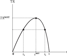
Figure 7.1 The Laffer curve

It is important, in studying Figure 7.1, to keep in mind that t^MAX is not necessarily the optimal t. The optimal t will balance out the benefits that a further rise in t would confer against the costs that it would impose. Imagine that the government has set t at t₁ and that it is considering a small rise in t. The question is whether the value of the additional government spending made possible by that rise in t would more than offset the harm inflicted by the resulting fall in Y. If not, then it should not raise t. Conversely, it should consider whether the good made possible through the resulting rise in Y would more than offset the harm, through reduced government spending, of a reduction in t. If so, then it should reduce t. Only if neither a rise nor a fall in t is called for, on that line of thinking, has the government imposed the optimal t.

It is important to keep one more point in mind as we proceed. That point is that there is a huge difference between two kinds of tax law changes: those that affect the reward for choosing work over leisure or for choosing saving over consumption, on the one hand, and those that simply make the taxpayer poorer or richer, on the other. Probably the best examples of tax changes that exerted little influence on the rewards for work or saving were the tax rebates that were sent out under the administration of George W. Bush for the purpose of stimulating the economy.

If the government sends you a check in the mail, it can call that a tax rebate but it has exactly the same effect on your work–leisure decision or your saving–consumption decision that would occur if you received a lottery winning or a distribution from the estate of your late Aunt Edna whom you never knew very well. It just makes you richer without affecting the reward for putting another hour into work or another dollar into saving.

A check in the mail or any economic windfall produces a pure “income effect” of the kind discussed in Chapter 3. Although economic windfalls do affect the work–saving calculus, they do not affect it by making work or saving more or less attractive relative to leisure or consumption “at the margin.” They do not affect the reward for choosing another hour of work over another hour of leisure or for choosing another dollar of saving over another dollar of consumption. In other words, they do not exert substitution effects. They simply make current leisure and current consumption look more attractive.

Conversely, if the individual gets a bill in the mail for some amount of money that is unrelated to his reward for working another hour or saving another dollar, it affects his work–saving calculus only by making him feel poorer. The bill makes current leisure or consumption less attractive.

In Volume II, Chapter 3, we will see that the effects of tax changes under nonclassical conditions—say, a prolonged period of low production and employment—depend on how those conditions came about. Because there is a long-standing assumption that an economic downturn reflects general excess supply and because Keynes predicated his economic remedies on that assumption, tax rebates are often seen to be appropriate whenever the economy falls into a prolonged downturn. But we will see that an economy can fall into a prolonged downturn for reasons opposite of what Keynes assumed—say, for reasons stemming from general excess demand—and that the provision of economic windfalls through tax rebates may therefore be exactly the wrong remedy.

In this chapter we assume the existence of classical conditions, under which a gain or loss of cash, separate from any change in the reward for work or saving, exerts an income effect and that this income effect is registered under conditions in which aggregate supply equals aggregate demand. We will proceed on the assumption that there is no Keynesian excess supply or, conversely, any suppressed-inflation type excess demand, to worry about. We relax these assumptions in Volume II.

Tax laws exert many effects on behavior beyond their direct income effects. Take a look at your IRS Form 1040. If you subtracted “education expenses” to compute your adjusted gross income, then the availability of that deduction probably influenced your education spending. The deduction for “alimony” paid might even affect your decision to get divorced or not (which one can hope you didn’t have to do). Other items (deductions for student loan interest, charitable expenses, and personal exemptions) influenced other choices, which, presumably, they were intended to do. Some of these features of the law do impose substitution effects but these are so hard to separate from their income effects as to make it difficult to fit them into an analysis of how tax law affects the overall economy. It is therefore useful, in studying macroeconomics, simply to treat such deductions as if they were just “checks in the mail,” every bit the same as tax rebates.

Our job here is to understand how tax changes affect the economy and to do so by understanding how they affect decisions to supply and use labor and capital. We begin by considering labor.

Taxes on Labor Income

Recall the discussion of substitution and income effects in Chapter 3, which we have considered in Figure 7.2. In this example, Adam saw his wage rise from $50 to $100 per hour, only to have his boss extort $500 in income from him as his wage rose. There we saw that Adam would allocate more time to work at the new wage rate if he had to pay this extortion than if he did not. The extortion took away the income effect that would otherwise have led Adam to consume more leisure.

Now let’s approach this situation from the other way around, and let’s let the government take on the role of Adam’s boss. Adam starts out by working 12 hours a day and making $100 per hour in labor income. Then the government imposes a 50% tax on his income so that his after-tax wage rate falls to $50 per hour. He increases leisure by two hours from 12 to 14 hours per day, reducing his work from 12 to 10 hours per day. Of the $1,000 in before-tax income that he now earns, he pays $500 to the government, leaving the rest in after-tax labor income. His utility falls from U₂ to U₁.

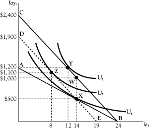
Figure 7.2 Effect of a tax on labor income

The adjustment in his work effort is the product of competing substitution and income effects. Because his after-tax wage rate falls by 50%, the cost of leisure also falls by 50% and Adam, to that extent, wants more leisure. But he must also pay $500 in taxes on his $1,000 in before-tax income, as shown by point W, which means that he can afford less leisure than before. The income effect on work and leisure results from the downward shift of $500 by the budget line from BC to DE and the shift from point Y to point Z. The substitution effect is illustrated by the shift from point Z to point X. Adam reduces his leisure time (and increases his work time) by four hours because of the income effect and increases his leisure time (and decreases his work time) by six hours because of the substitution effect. The net expansion in leisure time (and contraction of work time) by two hours is the net result of these competing effects.

In this example, the work-increasing income effect of the tax offsets much of the work-decreasing substitution effect. It seems, in light of this example, that a tax on labor income might cause only a small reduction in the supply of labor. Conversely, the removal or reduction of a tax on labor income might cause only a small increase in labor supply.

The discussion of Chapter 3 brings another point to light. Suppose that the government decided to collect its $500, not by taxing labor income, but by simply sending Adam a bill for $500, which he would have to pay irrespective of his work–leisure choice. It imposes what we call a lump-sum tax. This would be akin to the hypothesized “donation” that his boss expected him to make in the example of that chapter. After he pays the government, Adam gets to keep the entire $100 in pay that he receives for every hour he works.

As in Chapter 3, we illustrate that eventuality by a shift inward of his budget constraint from BC to ED. This action eliminates the substitution effect since it leaves take-home pay (once the tax bill is paid) unchanged. The cost of leisure does not go down and as a result there is no inclination on that account to substitute leisure for work. All that is left is the income effect, which, since Adam feels poorer now than he did at point Y, induces him to reduce his leisure from 12 to 8 hours (and increase his work from 12 to 16 hours) as he shifts from point Y to point Z. There is an argument from the economic efficiency viewpoint to go from the existing tax system to a more neutral tax under which income effects replace substitution effects in this manner. Adam is better off at point Z than he would be at point X. It also happens that his work time rises by four hours rather than falling by two hours as it does under the income tax.

Interestingly, this argument flies in the face of the “folk-economic” view that the harm from taxes results from the fact that they “take money out of people’s pockets.” But the harm is greater under an income tax than under a lump-sum tax. Either tax takes the same amount of money out of the taxpayer’s pockets, but the income tax imposes an additional harm by reducing the cost of leisure and thereby inducing the taxpayer to increase leisure, in which case he ends up worse off than he would have been under a lump-sum tax.

We reach the conclusion that the economic effect of a tax depends on just how it is assessed. But it also depends on how government uses the tax revenue it raises. The forgoing analysis disregards this question entirely. It assumes, in effect, that that government takes $500 of Adam’s money— money that would otherwise have gone toward the purchase of useful consumer goods—and applies it to some entirely wasteful project. Perhaps the government pays workers to dig holes in the ground and fill them in again, diverting those workers from the production of previously enjoyed consumer goods. (Oddly, this possibility would work just fine in an economy characterized by Keynesian excess supply, but recall that we are assuming that there is no imbalance between aggregate supply and demand.)

Figure 7.3 illustrates an alternative scenario, one in which the individual is subjected to a 50% income tax but nevertheless rises to a higher level of utility because of the value to him of the government services paid for out of the tax revenue raised by the tax. Suppose that service is the provision of “free” health care, for which Adam previously paid $600 out of his pocket. This can be thought of as a lump-sum benefit, which Adam gets without doing anything at all. This tax-benefit combination puts him on line EF. This line is based on the assumption that Adam can enjoy the $600 in consumption without working at all (point E). At the other extreme, he could enjoy $1,800 in consumption by working the entire 24 hours (point F).

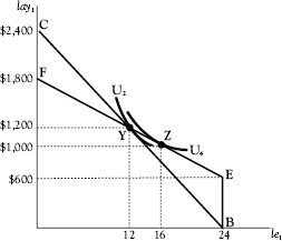
Figure 7.3 Effect of an income tax when tax revenue is not wasted

Now also Adam can have the same amount of consumption and the same amount of leisure that he had before the tax-benefit arrangement was instituted, which means that it permits him to return to point Y, where he has 12 hours of leisure and $1,200 in consumption and the same level of utility U₂. In actuality, because the tax makes leisure cheaper, he would adjust to point Z and to a higher level of utility U₄.

Interestingly now, the government raises less in revenue than it did when it wasted the money, the reason being that the $600 windfall partially offsets the income effect of the income tax, causing him to expand leisure by two hours more than he would have if the revenue had been wasted. Thus, he ends up working only eight hours and paying only $400 in taxes. His eight hours of work leaves him with $400 in after-tax income, which, plus the value of the government benefit, permits him to consume $1,000 worth of goods. (Keep in mind that, in this example, it must be possible for the government to provide the aimed-for $600 in services by raising only $400 in revenue.)

These examples relate to taxes on labor income, but they apply as well to taxes on capital income. They teach three lessons:

It is important to note that the example in which an increase in income tax yields beneficial forms of increased government spending posits spending of the kind that translates into an equivalent reduction in the cost of some item on which the individual already spends. The converse example would be a tax cut that requires the individual to spend his tax saving on something previously provided “free” by the government. Because plausible examples are hard to find, it seems likely that income taxes will exert income as well as substitution effects. Also, the substitution effect will more and more dominate the income effect as the tax rate approaches 100%.

The next question is how the imposition of an income tax will affect the demand for labor. Again, suppose that there is no income tax and Adam has a job that pays $50 per hour. We know from Chapter 5 that Adam will adjust his work effort so that

and his employer will adjust the quantity of labor purchased from Adam so that

Thus, as shown in Chapter 6, the socially optimal amount of labor is provided, inasmuch as

the income generated by another hour of labor time is just equal to the income that Adam would have to receive in order to be willing to provide that hour of labor time.

Now suppose the government imposes a 50% tax on labor income. Adam’s after-tax wage rate w_at now equals 50% of his before tax wage rate w_bt:

Because he adjusts his work effort to his after-tax wage, he will set

while his employer sets

It follows that

The wage that Adam would have to receive, after taxes, in order to provide another hour of labor time is less than the additional income that the firm would receive by using that hour of labor time. As a result, the firm hires less than the socially optimal quantity of labor. As previously observed, the tax on labor income imposes a bias in favor of leisure and against work (see Figure 7.4).

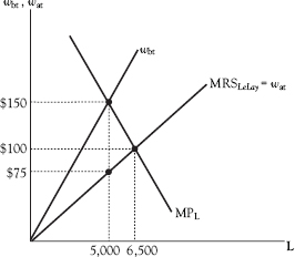
Figure 7.4 Effect of an income tax on the supply of labor

Without a tax, the quantity of work time hired by firms would be 6,500 hours at $100 per hour. Under a 50% income tax, the labor supply curve rotates in a counterclockwise direction so that the before-tax wage rate now diverges from the after-tax wage by $75 per hour. The quantity of labor hired falls to 5,000 hours, and the government collects $375,000 (= $75 × 5,000) in revenue.

Taxes on Capital Income

Capital income is a reward for saving. Our hypothetical taxpayer has a certain amount of disposable income, which she—we are bringing Eve back into the story—uses either for consumption or saving. She saves by using after-tax income to buy saving instruments like bank CDs, bank passbook saving accounts, government or corporate bonds, or corporate stocks. (She can also save by putting her money in a cookie jar, but that doesn’t create any taxable capital income.) What she doesn’t save, she uses for consumption or to pay taxes.

Earlier in this chapter, we expanded the framework of Chapter 3, where the individual had a certain amount of labor income that he had to divide between current and future consumption, to a revised framework in which the same individual had to take into account any taxes that were imposed on labor income.

Here we expand the framework of Chapter 4, where the choice between current and future consumption depends on r, ρ, and the individual’s IES, to a revised framework that takes into account taxes that are imposed on capital income. We do so by introducing taxes on the income made possible by saving. Savers receive capital income by making financial capital provided through bank deposits and corporate stock and bond purchases available to firms. (For this purpose, we ignore institutions that provide financial capital.)

Businesses use financial capital provided through saving to engage in capital spending, that is, investment. In Chapter 5 we assumed that savers provided financial capital only through loans, which could be made via banks or directly to business investors. Here we expand the analysis to include financial capital provided via stock purchases.

In Chapter 5, the equilibrium r was determined through the interaction of a lender (Eve) and an investor (Adam). Recall that, in classical equilibrium, investment would expand until the marginal product of capital equals the real interest rate plus economic depreciation:

where r + d equals the cost of capital cc.

Now let’s consider what happens when the government imposes a tax t on interest income. We return to the Garden of Eden, after the fall, where Eve saves and Adam invests. In Chapter 5, we considered the conditions that would have to be met in order for Adam and Eve to reach equilibrium in their saving–investment calculus. But now we have to think about how the imposition of this tax might affect the cost of capital cc and what we will call the after-tax return to saving r_at. Let the before-tax interest rate enjoyed by Eve, which is to say, the interest rate that Adam actually pays, be r_bt. Then

In order for Eve’s after-tax return on her saving to match the return r she got before the tax was imposed, r_bt must be high enough so that r_at = r. Thus it must be true that

What does this mean for the cost of capital? The answer is that it depends on whether Adam can deduct the cost of capital from his taxable income. Suppose that Eve passes on the full amount of the tax to Adam by charging the interest rate r_bt as defined in equation (7.12), and suppose that Adam can deduct both the interest he pays Eve and economic depreciation. (In fact, the amount of depreciation that can be deducted will differ from economic depreciation, but we ignore this distinction for now.) If Adam’s business income is taxed at the same rate as Eve’s interest earnings are taxed, then cc becomes

There is no effect on the cost of capital if Adam uses debt financing to acquire the funds needed to buy his oven and if depreciation and the cost of debt financing is fully deductible.

Now let’s examine what Eve is doing about her saving decision. Eve adjusts her saving until

For his part, Adam adjusts his capital holdings until

Because

which we previously saw as equation (5.31) in Chapter 5.

The value to the firm of another dollar of capital spending is just equal to the increment in future consumption that a saver would have to receive in order to make a dollar available to the firm for the purpose of buying new capital.

Taxing Corporate Income

The matter becomes more complicated when Adam obtains financing by offering ownership in the firm rather than by just borrowing the money. The traditional arrangement is to form a corporation and use equity capital (i.e., sell stock) to finance capital purchases.

Let’s assume that the after-tax return to Eve for providing debt financing is 5% and that Adam already has four pizza ovens for his business but now wishes to secure equity financing to buy a fifth oven. He wants to make a stock offering that will bring in enough cash so he can buy an oven costing $1,000, which, we assume, depreciates at the rate of 10% per year. Adam plans to sell the stock to Eve and to compensate her for her stock purchase by paying out the entire return on the additional oven as a dividend.

If there were no taxes to be paid on this return and if Eve’s stock purchase were for $1,000, Adam would pay her an annual dividend of $150, which would be just high enough to cover her expected after-tax return of 5% plus another 10% to cover the annual loss in share value owing to the depreciation of the oven.

However, there will be taxes to pay, which makes all the difference between this and the arrangement in which Adam relied on debt financing. In fact, there will be two taxes to pay as the profit generated by the purchase of the fifth oven makes its way to Eve’s pockets. First there is the corporation income tax, imposed at a rate of t_c, which we will assume to be 21% (which is the top statutory rate on U.S. corporations). Then there is the individual income tax rate, t_div, that Eve will have to pay on the dividends she receives, which in her assumed tax bracket, would be 15%. (There would ordinarily be a state corporation income tax for Adam to pay and a state income tax for Eve to pay, but we will ignore those taxes here.)

So the question is what rate of return would Eve have to get on her stock in order to make it worth her while to buy that stock rather than put her money in the bank. This rate of return is now the cost of capital to Adam, in this instance the cost of raising financial capital by selling stock. As before, we will designate this cost of capital as cc. In order to determine cc, we need to figure out how much in taxes Adam and Eve will have to pay before Eve sees a dollar of reward for buying stock in Adam’s company.

Let’s start with the tax treatment of depreciation on the oven. If the IRS lets Adam depreciate the oven over a period of five years, he will be able to reduce his company’s taxable income by 1/5 of $1,000, or by $200, for five years after he buys the oven, beginning with the first tax year for which he can take the depreciation. At a tax rate of 21% (per the Tax Cuts and Jobs Act of 2017), that’s an annual saving of $42 (= 0.21 × $200). If the discount rate is 5%, the present value of this saving is

In effect, the depreciation allowance reduces the cost of buying the oven by 18.18%, from $1,000 to $818.16.

We will designate the fraction of the cost of buying a capital asset that the investor saves by depreciating that asset as f_d. (here equal to 18.18%). We will ignore any tax saving that Adam might enjoy by taking advantage of an investment tax credit or some other such benefit that the tax laws might allow.

The fact that Adam can depreciate his capital for tax purposes makes it cheaper for him to raise financial capital. Let’s imagine that the tax laws permitted Adam to depreciate a new oven in the manner just described. Because Adam would, we also assume, have to pay corporate taxes on income yielded by other investments, he could still reduce his overall tax liability by $42 for each of the next five years just as we previously noted. Adam could use the resulting stream of tax savings to reduce the amount of financial capital he needs to raise in order to buy the oven. Thus in this example, he needs to raise only $818.16.

Now let’s see where we are in computing the tax burden on Adam’s business and on Eve’s pocketbook that results when she provides enough financing in order for him to buy the oven. First, if the oven generates a profit, his corporate tax liability for receiving the income generated by the purchase of the oven will be

where t_c is the corporation tax rate that applies to income generated by this purchase. Because Adam distributes all of his after-tax corporate income as dividends, Eve gets a before-tax dividend equal to

So

Eve will pay a tax on her dividend of

Her after-tax dividend will then be

We know that Eve has to end up with an after-tax dividend high enough to justify taking $818.16 out of the bank and using it to buy pizza stock. That after-tax dividend is

In order for Eve to receive this after-tax dividend, Adam must receive income from the purchase of the oven of

Using the information we have about this investment, the income Adam must receive is

The pizza oven must generate a profit of $182.76 in order to leave Eve with her required after-tax dividend. Adam’s corporation pays 21% or $38.38 in taxes on its income, leaving it with $144.38 in after-tax income to be distributed to Eve as a dividend, on which she pays taxes of $21.66 (= 0.15*144.38), leaving her with $122.72, which is required after-tax income. Because $122.72/818.16 = 15%, this leaves her with just enough to earn a 15% return on her purchase of $818.16 worth of Adam’s Pizzeria stock.

The cost of capital to Adam is

or, in this instance,

The investment must yield a return of 18.27% to make it worthwhile for Eve to furnish her equity capital. We can compute the marginal effective tax rate on her stock purchase as

Note that total taxes are $60.04, which is 32.82% (before rounding) of the $182.76 in income that the project needs to generate.

We can illustrate this graphically if we translate the forgoing results into their consequences for capital spending. See Figure 7.5. We have found that the cost per dollar of financial capital needed for Adam to buy a pizza oven is 18.27¢, of which 32.82%, or 6¢, is paid in taxes. This means that savers receive only 12.27¢ after taxes, for every dollar of capital expenditure.

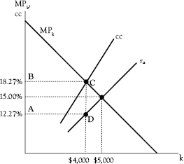
Figure 7.5 Effect of a corporation income tax on the capital stock

The cost of capital would be 15% but for the tax, in which case the firm would want to have five ovens, inasmuch as MP_k = 15% when k = $5,000. Instead the firm acquires only four ovens. The government receives 6¢ in taxes for every dollar of capital held by the firm, which in this example comes to $240, which is the size of area ABCD.

Table 7.1 provides some alternative computations of the cost of capital and the marginal effective tax rate (METR) for different assumptions about depreciation, the corporate tax rate, and the tax rate on dividends. One scenario sets the corporate tax rate at 35%, where it stood before the Tax Cuts and Jobs Act of 2017. A second lengthens the depreciation period to 15 years under current law. The last sets the dividend tax rate at 20%, which is the top rate under current law.

We see that the cost of capital rises with the dividend tax rate, the corporate tax rate, and the length of the depreciation period. The greater the cost of capital, the smaller the desired number of pizza ovens. This has implications for economic activity in that GDP is larger the larger the capital stock.

Now let’s return to our current-law scenario, in which the corporate tax rate was 21%, the tax rate on dividends was 15% and the depreciation period was five years. As shown in Figure 7.5, the firm adjusts its capital stock until

Table 7.1 Effects of alternative tax rates and depreciation periods

Given			We can calculate cc and METR as follows:
Dividend tax rate (%)	Corporate tax rate (%)	Depreciation period (years)	Cost of capital (%)	Marginal effective tax rate (%)
15	35	5	18.92	44.75
15	21	10	18.72	32.87
20	21	5	19.42	36.80

The saver offers financial capital only up to the point where

Thus in this example,

Equation (7.17) is not satisfied: The value to the firm of adding another dollar of capital is greater than the amount of future consumption with which savers would have to be compensated for providing that additional dollar. The taxes create a bias toward consumption and away from saving. In Figure 7.5, that bias is enough to discourage the firm from buying the fifth oven.

Untaxing Net Investment

Another approach to tax policy is to identify tax-rate changes that would keep tax revenues constant (i.e., be “revenue neutral”) but nevertheless expand the economy. One way to do that would be to repeal the tax on income and replace it with a tax on consumption that is just high enough to keep revenues constant.

To see how this would work, let’s begin with our stripped-down version of the NIPA income-expenditure equality from Chapter 2:

The left-hand side is wages plus nonwage income plus depreciation of private capital, and the right-hand side is the sum of all expenditures that make up GDP. Let’s assume, for this purpose, that nonwage income is asset income.

Under the income tax, the tax base is wage plus nonwage income, which is to say the left-hand side of equation (7.34).² Subtracting depreciation from both sides of the equation, we get

National income and product accounting provides a reminder that taxes imposed on the income side of the equation, which is the left-hand side of equation (7.35), must fall equally on the expenditure side, which is the right-hand side.

Suppose, to begin with, that taxes are imposed on both wage and nonwage income and that Adam’s pizza business has $1,000 in profits. In the preceding example, he would pay $210 in corporate income taxes. He would then have $790 left, which he could use to buy new capital or distribute to Eve in the form of dividends. If he chose to distribute the profits to Eve, she would, for her part, pay $118.50 (= 0.15 × ($790)) in taxes on her $790 in dividends. Adam’s $1,000 in profits would leave Eve with $671.50 in after-tax income. The government would collect $328.50 (= 32.85% of the $1,000 in profits) in revenue.

Now suppose that the government decides to tax only labor income. The tax base would be LAY or what we called “labor income” in Chapter 2. If Adam receives $1,000 in profits, he could distribute that amount to Eve in dividends, on which she would pay no taxes. Adam’s $1,000 in profits would leave Eve with $1,000 in after-tax income, which she could apply either to consumption or to saving in the form of providing more financial capital to Adam. If she chose to use the same $1,000 to buy stock from Adam, he would be able to apply that entire amount to the purchase of a new capital, as if he had not distributed the profits to Eve in the first place. The tax base would be

Suppose, alternatively, that the government taxed both wage and non-wage income but permitted firms to deduct capital expenditures from their taxable income. This is known as “expensing” investment. The tax base would be

Note that, if NW = Net I, which would be the case if Adam used Eve’s $1,000 to buy new capital, the tax base is the same, whether defined according to equation (7.36) or equation (7.37). Either way, it untaxes net investment, and the tax has the sole effect of reducing after-tax wages.

We can also rewrite equation (7.37) as follows, so that the tax falls only on C and G and that net exports are also untaxed:

Were net exports to equal zero, the policies would yield the same tax base.

The policy of permitting firms to expense net investment is the core feature of flat tax proposals, notably those put forward by Robert Hall and Alvin Rabushka and by Steve Forbes (Hall and Rabushka 2007; Forbes 2005). The left-hand side of equation (7.37) provides the flat tax base. The best-known proposal for a consumption tax is the “FairTax,” which would tax consumption through a national retail sales tax. The left-hand side of equation (7.38) provides the FairTax base.

Despite the hot dispute that can arise between “flat taxers” and “fair taxers,” the two ideas have in common the fact that they untax net investment, which is the crucial consideration for tax policy. The argument for this policy lies in the expectation that the expansive effect of untaxing net investment would more than offset the contractive effect of raising the tax on labor. Both approaches pose some issues for the monetary authorities, which issues we take up in Volume II, Chapter 1.

Evidence

David and Christina Romer argue persuasively that tax increases generally have negative economic effects:

In another study, Romer and Romer conclude from the evidence “that taxes are indeed distortionary: the null hypothesis of no effect is overwhelmingly rejected.” On the other hand, they find that “the distortions are small.” Their “baseline estimate of the elasticity of taxable income with respect to the after-tax share is approximately 0.2. This is considerably smaller than the findings of postwar studies (though generally within their confidence intervals). Finally, the estimates are extremely robust” (C. D. Romer and Romer 2013, p. 39).

In a study on How the Supply of Labor Responds to Changes in Fiscal Policy, the Congressional Budget Office contrasted the effects of short-term and permanent tax changes:

For a permanent tax change, the result is far less robust:

Mathias Trabandt and Harald Uhlig estimated the Laffer curve for the United States and a group of 14 European Union countries. They found that

On the basis of this finding, the United States could expand the economy and increase tax revenues by untaxing net investment.

Having considered the effects of taxes on the economy, we turn next to the government expenditures for which taxes are imposed.

¹ Senator Elizabeth Warren of Massachusetts did once suggest that the minimum wage should be $22 an hour. See Senator Elizabeth Warren, “Minimum Wage Would Be $22 An Hour If It Had Kept Up With Productivity,” 2013. Retrieved August 18, 2013, from http://huffingtonpost.com/2013/03/18/elizabethwarren-minimum-wage_n_2900984.html

² In reality the existing income tax provides numerous deductions for nonwage income and is, therefore, a kind of compromise between a “pure” income tax and a consumption tax.

³ Note that we assume that the tax would apply personal consumption expenditures and to all government purchases, not just the portion identified as government consumption expenditures in the NIPA.

⁴ In any discussion of tax policy, it is important to distinguish marginal tax rates from average tax rates. Consider a married couple who set out to calculate their 2017 federal income tax bill, and suppose that they find that their 2017 taxable income was $150,000. Using the IRS tax tables we find that they owe the government $29,466. Their average tax rate equals their tax bill divided by their taxable income, or 19.64%. But their marginal tax rate is 28%, given that they find themselves in the 28% income tax bracket. The distinction is important for assessing how their tax schedule affects their willingness to work. Suppose that our couple (Adam and Eve, of course) had to decide on January 1, 2018, whether one of them should take a consulting job that would pay $3,600. Because taking that job would push them into the 28% tax bracket, they must compute the after-tax reward for taking that job on the assumption that doing so would add $1,008 (= 0.28 × $3,600) to their taxes. What matters is their marginal, not their average tax rate. From this example, we see why economists who attempt to determine the effects of tax-law changes on economic behavior focus on changes in marginal, not average rates. Using evidence on changing average rates to measure economic effects is misleading because average rates are calculated by dividing tax liabilities by taxable income, which itself depends on how changes in marginal rates affect economic behavior.