Chapter 5
Step I
Objective Assessment
When you receive digital files for mastering, you must first verify and notate seven objective assessment parameters that reveal critical aspects of the audio file. This preliminary data will begin to inform your game plan or strategy to effectively master the project.
In this era of music production, the vast majority of mix files a Mastering Engineer receives are digital files. The stark reality remains that today, the number of clients who provide me with analog master tapes is negligible. And, although it represents an excellent format—with the appealing sound coloration of tape compression—the added cost and time have made mixing to tape nearly obsolete. Whereas objective assessment should also be done for an analog source via analog VU/peak meters, for the reasons just mentioned, I will focus on digital source files.
Verify the Sampling Frequency (S), Bit Depth (BD), and File Type
Never take the client’s word about the sampling frequency (S) and bit depth (BD) of a source file. It remains your responsibility to verify all aspects of the digital source. A working knowledge of sampling theorem (see definition in Chapter 1 under Key Understandings to Possess) remains essential to understand the implications of the digital portion of objective assessment. A Mastering Engineer must understand three critical parameters that originate from sampling theorem and the information they indicate: sampling frequency pertains to the bandwidth of the audio; bit depth pertains to the dynamic range of the audio; and multiplying the S, BD and the number of channels of audio yields the bit rate in kilobits-per-second (kbps).1 The Nyquist frequency2 (S/2) is one-half the S and determines the audio bandwidth of the file. For instance, a file with a S of 44.1kHz has a Nyquist frequency of 22.05kHz—meaning there will be no audio sampled and reproduced above 22.05kHz.
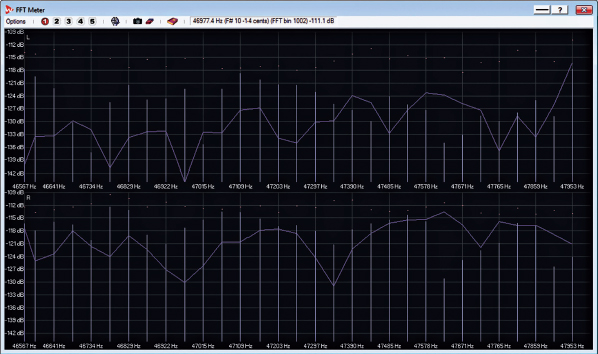
Use the onboard tools or third-party plug-ins in your DAW to verify these properties of the digital audio file. For instance: in Pro Tools (Figures 5.1 and 5.2), window menu then workspace displays S and BD; on a PC right click then select properties to display the bit rate from which the S and BD can be extrapolated using simple arithmetic. WaveLab (Figure 5.3) has an onboard bit meter to verify bit depth (or use a bit meter plug-in such as Bitter [Figure 5.4]), a spectrum analyzer to verify frequency response (and thus the Nyquist frequency), and loudness meters to verify level. Or, open the .wav file in WaveLab (Figure 5.5), and the S and BD will display in the lower right corner of the main display. Use these tools to verify the parameters/formats of flat mix files, raw mastered files or files rendered for final delivery. Finally, notate the S, BD, and the file type provided to compile three of the seven parameters of objective assessment.
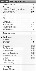
Figure 5.1In ProTools, select Window→Workspace from the menu.


Measure the Decibels Full Scale (dBFS) RMS and Peak Levels of the Audio File
These two criteria represent the fourth and fifth of the seven objective assessment parameters. All DAWs have onboard tools whereby you can take these measurements. In Pro Tools, under the Audiosuite menu, the Gain plug-in has an analyze button that will measure and display these readings for a highlighted file (Figure 5.6). In WaveLab, under the Analysis menu item, there is a global analysis (keystroke ‘y’) dialogue box to check the readings of the mastered file (Figure 5.7). Notate these readings, along with the S and BD. Additionally there are a number of effective metering plug-ins to choose from to obtain this information: Voxengo SPAN (Figure 5.8), Brainworx bx_meter, HOFA 4U Goniometer & Korrelator, iZotope Insight, Waves Dorrough, and FabFilter Pro-L 2 are all good options.

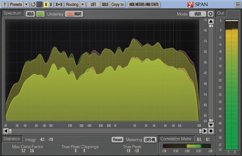
Figure 5.8The Voxengo SPAN plug-in will do spectrum analysis and loudness metering.
Source: (courtesy Voxengo)
These readings will provide immediate information about how the song was mixed, if the mixer used a peak-limiter, and if it is dynamic enough for an effective mastered result (or if it is already too peak-limited with problematic artifacts). If it means a better sounding final master, don’t shy away from requesting more dynamic, less peak-limited mix files to work from.
VU Meter Reading
Whereas the five digital objective assessment parameters discussed previously (S, BD, dBFS RMS, dBFS Peak, and file type) can be ascertained via computer algorithms—the sixth parameter, an analog VU meter reading—must occur in real time. Analog VU meter levels (indicated in dBu) remain excellent for assessing level in audio recordings, particularly in mastering. A VU meter is an analog device calibrated to measure electronic voltage levels, and the ballistics of the meter needles react more to average levels of the audio, so they measure the root mean square (RMS) of the continuous audio signal. VU meter ballistics closely approximate the response of human hearing, and remain useful for verifying level cohesion from song to song, and to ensure the album won’t be too loud for downstream applications. Carefully listen to the flat mix for fidelity, and also pay close attention to your VU meters as it plays. Notate the loudest levels, usually in choruses or large endings. If, for example, these sections read +6dBu, this is your starting point for mastering—it provides an exact indication of the total gain required through your mastering system to achieve the desired target level. See Chapter 1, Figure 1.6, for an example of VU meters.
Target Levels of Mastered Audio
The various music genres possess specific target levels once mastered. These represent unofficial guidelines that I’ve compiled over many years of mastering a wide variety of musical genres. You can conduct your own target level research by performing objective assessment on your favorite (or charting) recordings.
VU meters provide practical information about the average loudness of both the source mix and the mastered audio. Using VU meters on both source audio and the mastered result allows for a quick real-time calculation of the gain added through the mastering system. Achieving the desired target level for the mastered audio represents a crucial aspect of the mastering session.
| Genre | Target Level (VU) |
|---|---|
| Rock (and most sub-genres) | +12dBu—+13.5dBu |
| Pop (and most sub-genres) | +13dBu—+14dBu |
| Singer/Songwriter | +12dBu—+13.5dBu |
| Hip-Hop/Rap | +14dBu—+15dBu |
| EDM/Dance | +14dBu—+15dBu |
| Jazz | +9dBu—+11dBu |
| Non-Limited High-Resolution Audio (HRA) | +6dBu—+8dBu |
Waveform Inspection
This represents the seventh and final parameter of objective assessment. Upon opening the mix file in your PBDAW, you will notice the waveform display. Does it resemble a forest, with many jagged peaks visible? If so, chances remain high that transients are intact and it represents a dynamic mix file. This observation should be supported by the other measured objective assessment criteria outlined previously—especially a dBFS Peak less than 0, and an RMS reading below −15dBFS. Zoom into the waveform: Are the peaks rounded rather than flat? If so, this represents additional evidence of a dynamic mix with little or no peak-limiting.
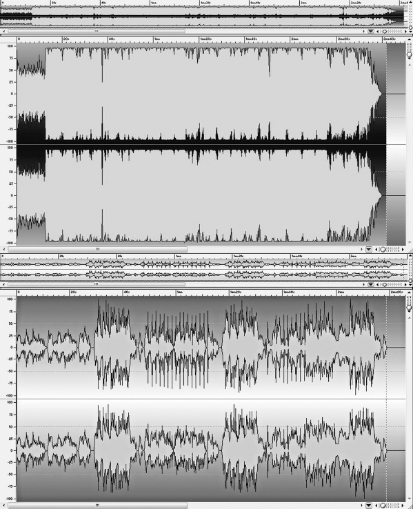
However, if your mix file looks like a block, and when you zoom in the peaks are sometimes sheared off like a butte, then you are looking at a loudness-maximized or peak-limited mix (Figure 5.9). Again, the other objective assessments should support this observation—meaning a dBFS Peak of 0 (or between −0.1 and −0.3), and an RMS reading above −15dBFS. If the mix is already at the target level, ask the client for a less peak-limited file. If the engineer mixed with the peak-limiter on the stereo buss, have them back down the amount of limiting but leave the device on, as many mix balance decisions were likely made with it on.
Conclusion
This completes our study of the seven parameters of objective assessment, which establish the fundamental scaffolding of the mastering process. This includes how much gain is required through the mastering system to achieve the chosen target level, and what approach to adopt given the degree of dynamic range in the source mix. Next, I will explore Step II of The Five Step Mastering Process, subjective assessment. Together, these two assessment processes equip the Mastering Engineer with the data and observations to understand the strengths and weaknesses of the mix file, and decide on the optimal approach to appropriately master the audio for the highest possible fidelity.
Exercises
- Perform objective assessment observations on a mix file and notate the seven criteria outlined in this chapter (S, BD, file type, dBFS Peak, dBFS RMS, VU Level, and waveform inspection).
- Perform objective assessment observations on the mastered version of the same file and notate the seven criteria. Compare how the following level parameters changed (dBFS Peak, dBFS RMS, VU meter reading, and waveform display). Write a few sentences explaining the changes and what they indicate.
- Explain what sampling frequency (S) and bit depth (BD) reveal about a digital audio file.