3

High Availability and Reliability

In Chapter 2, Creating Kubernetes Clusters, we learned how to create Kubernetes clusters in different environments, experimented with different tools, and created a couple of clusters. Creating a Kubernetes cluster is just the beginning of the story. Once the cluster is up and running, you need to make sure it stays operational.

In this chapter, we will dive into the topic of highly available clusters. This is a complicated topic. The Kubernetes project and the community haven’t settled on one true way to achieve high availability nirvana. There are many aspects to highly available Kubernetes clusters, such as ensuring that the control plane can keep functioning in the face of failures, protecting the cluster state in etcd, protecting the system’s data, and recovering capacity and/or performance quickly. Different systems will have different reliability and availability requirements. How to design and implement a highly available Kubernetes cluster will depend on those requirements.

This chapter will explore the following main topics:

• High availability concepts
• High availability best practices
• High availability, scalability, and capacity planning
• Large cluster performance, cost, and design trade-offs
• Choosing and managing the cluster capacity
• Pushing the envelope with Kubernetes
• Testing Kubernetes at scale

At the end of this chapter, you will understand the various concepts associated with high availability and be familiar with Kubernetes’ high availability best practices and when to employ them. You will be able to upgrade live clusters using different strategies and techniques, and you will be able to choose between multiple possible solutions based on trade-offs between performance, cost, and availability.

High availability concepts

In this section, we will start our journey into high availability by exploring the concepts and building blocks of reliable and highly available systems. The million (trillion?) dollar question is, how do we build reliable and highly available systems from unreliable components? Components will fail; you can take that to the bank. Hardware will fail, networks will fail, configuration will be wrong, software will have bugs, and people will make mistakes. Accepting that, we need to design a system that can be reliable and highly available even when components fail. The idea is to start with redundancy, detect component failure, and replace bad components quickly.

Redundancy

Redundancy is the foundation of reliable and highly available systems at the hardware and software levels. If a critical component fails and you want the system to keep running, you must have another identical component ready to go. Kubernetes itself takes care of your stateless pods via replication controllers and replica sets. But, your cluster state in etcd and the control plane components themselves need redundancy to function when some components fail. In practice, this means running etcd and the API server on 3 or more nodes.

In addition, if your system’s stateful components are not already backed up by redundant persistent storage (for example, on a cloud platform), then you need to add redundancy to prevent data loss.

Hot swapping

Hot swapping is the concept of replacing a failed component on the fly without taking the system down, with minimal (ideally, zero) interruption for users. If the component is stateless (or its state is stored in separate redundant storage), then hot swapping a new component to replace it is easy and just involves redirecting all clients to the new component. But, if it stores local state, including in memory, then hot swapping is not trivial. There are two main options:

• Give up on in-flight transactions (clients will retry)
• Keep a hot replica in sync (active-active)

The first solution is much simpler. Most systems are resilient enough to cope with failures. Clients can retry failed requests and the hot-swapped component will service them.

The second solution is more complicated and fragile and will incur a performance overhead because every interaction must be replicated to both copies (and acknowledged). It may be necessary for some critical parts of the system.

Leader election

Leader election is a common pattern in distributed systems. You often have multiple identical components that collaborate and share the load, but one component is elected as the leader and certain operations are serialized through the leader. You can think of distributed systems with leader election as a combination of redundancy and hot swapping. The components are all redundant and when the current leader fails or becomes unavailable, a new leader is elected and hot-swapped in.

Smart load balancing

Load balancing is about distributing the workload across multiple replicas that service incoming requests. This is useful for scaling up and down under a heavy load by adjusting the number of replicas. When some replicas fail, the load balancer will stop sending requests to failed or unreachable components. Kubernetes will provision new replicas, restore capacity, and update the load balancer. Kubernetes provides great facilities to support this via services, endpoints, replica sets, labels, and ingress controllers.

Idempotency

Many types of failure can be temporary. This is most common with networking issues or with too-stringent timeouts. A component that doesn’t respond to a health check will be considered unreachable and another component will take its place. Work that was scheduled for the presumably failed component may be sent to another component. But the original component may still be working and complete the same work. The end result is that the same work may be performed twice. It is very difficult to avoid this situation. To support exactly-once semantics, you need to pay a heavy price in overhead, performance, latency, and complexity. Thus, most systems opt to support at-least-once semantics, which means it is OK for the same work to be performed multiple times without violating the system’s data integrity. This property is called idempotency. Idempotent systems maintain their state even if an operation is performed multiple times.

Self-healing

When component failures occur in dynamic systems, you usually want the system to be able to heal itself. Kubernetes replica sets are great examples of self-healing systems. But failure can extend well beyond pods. Self-healing starts with the automated detection of problems followed by an automated resolution. Quotas and limits help create checks and balances to ensure automated self-healing doesn’t run amok due to bugs or circumstances such as DDoS attacks. Self-healing systems deal very well with transient failures by retrying failed operations and escalating failures only when it’s clear there is no other option. Some self-healing systems have fallback paths including serving cached content if up-to-date content is unavailable. Self-healing systems attempt to degrade gracefully and keep working until the core issue can be fixed.

In this section, we considered various concepts involved in creating reliable and highly available systems. In the next section, we will apply them and demonstrate best practices for systems deployed on Kubernetes clusters.

High availability best practices

Building reliable and highly available distributed systems is a non-trivial endeavor. In this section, we will check some of the best practices that enable a Kubernetes-based system to function reliably and be available in the face of various failure categories. We will also dive deep and see how to go about constructing your own highly available clusters. However, due to the complexity and the large number of factors that impact HA clusters, we will just provide guidance. We will not provide here step by step instructions for building a HA cluster.

Note that you should roll your own highly available Kubernetes cluster only in very special cases. There are multiple robust tools (usually built on top of kubeadm) that provide battle-tested ways to create highly available Kubernetes clusters at the control plane level. You should take advantage of all the work and effort that went into these tools. In particular, the cloud providers offer managed Kubernetes clusters that are highly available.

Creating highly available clusters

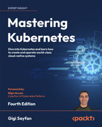
To create a highly available Kubernetes cluster, the control plane components must be redundant. That means etcd must be deployed as a cluster (typically across three or five nodes) and the Kubernetes API server must be redundant. Auxiliary cluster-management services such as the observability stack storage should be deployed redundantly too. The following diagram depicts a typical reliable and highly available Kubernetes cluster in a stacked etcd topology. There are several load-balanced control plane nodes, each one containing all the control plane components as well as an etcd component:

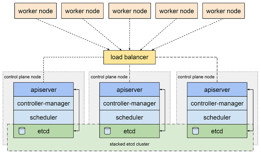
Figure 3.1: A highly available cluster configuration

This is not the only way to configure highly available clusters. You may prefer, for example, to deploy a standalone etcd cluster to optimize the machines to their workload or if you require more redundancy for your etcd cluster than the rest of the control plane nodes.

The following diagram shows a Kubernetes cluster where etcd is deployed as an external cluster:

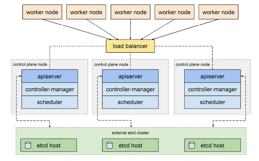
Figure 3.2: etcd used as an external cluster

Self-hosted Kubernetes clusters, where control plane components are deployed as pods and stateful sets in the cluster, are a great approach to simplify the robustness, disaster recovery, and self-healing of the control plane components by applying Kubernetes to Kubernetes. This means that some of the components that manage Kubernetes are themselves managed by Kubernetes. For example, if one of the Kubernetes API server nodes goes down, the other API server pods will notice and provision a new API server.

Making your nodes reliable

Nodes will fail, or some components will fail, but many failures are transient. The basic guarantee is to make sure that the runtime engine (Docker daemon, Containerd, or whatever the CRI implementation is) and the kubelet restart automatically in the event of a failure.

If you run CoreOS, a modern Debian-based OS (including Ubuntu >= 16.04), or any other OS that uses systemd as its init mechanism, then it’s easy to deploy Docker and the kubelet as self-starting daemons:

systemctl enable docker
systemctl enable kubelet

For other operating systems, the Kubernetes project selected the monit process monitor for their high availability example, but you can use any process monitor you prefer. The main requirement is to make sure that those two critical components will restart in the event of failure, without external intervention.

See https://monit-docs.web.cern.ch/base/kubernetes/.

Protecting your cluster state

The Kubernetes cluster state is typically stored in etcd (some Kubernetes implementations like k3s use alternative storage engines like SQLite). The etcd cluster was designed to be super reliable and distributed across multiple nodes. It’s important to take advantage of these capabilities for a reliable and highly available Kubernetes cluster by making sure to have multiple copies of the cluster state in case one of the copies is lost and unreachable.

Clustering etcd

You should have at least three nodes in your etcd cluster. If you need more reliability and redundancy, you can have five, seven, or any other odd number of nodes. The number of nodes must be odd to have a clear majority in case of a network split.

In order to create a cluster, the etcd nodes should be able to discover each other. There are several methods to accomplish that such as:

• static
• etcd discovery
• DNS discovery

The etcd-operator project from CoreOS used to be the go-to solution for deploying etcd clusters. Unfortunately, the project has been archived and is not developed actively anymore. Kubeadm uses the static method for provisioning etcd clusters for Kubernetes, so if you use any tool based on kubeadm, you’re all set. If you want to deploy a HA etcd cluster, I recommend following the official documentation: https://github.com/etcd-io/etcd/blob/release-3.4/Documentation/op-guide/clustering.md.

Protecting your data

Protecting the cluster state and configuration is great, but even more important is protecting your own data. If somehow the cluster state gets corrupted, you can always rebuild the cluster from scratch (although the cluster will not be available during the rebuild). But if your own data is corrupted or lost, you’re in deep trouble. The same rules apply; redundancy is king. But while the Kubernetes cluster state is very dynamic, much of your data may be less dynamic. For example, a lot of historic data is often important and can be backed up and restored. Live data might be lost, but the overall system may be restored to an earlier snapshot and suffer only temporary damage.

You should consider Velero as a solution for backing up your entire cluster including your own data. Heptio (now part of VMWare) developed Velero, which is open source and may be a lifesaver for critical systems.

Check it out here: https://velero.io/.

Running redundant API servers

The API servers are stateless, fetching all the necessary data on the fly from the etcd cluster. This means that you can easily run multiple API servers without needing to coordinate between them. Once you have multiple API servers running, you can put a load balancer in front of them to make it transparent to clients.

Running leader election with Kubernetes

Some control plane components, such as the scheduler and the controller manager, can’t have multiple instances active at the same time. This will be chaos, as multiple schedulers try to schedule the same pod into multiple nodes or multiple times into the same node. It is possible to run multiple schedulers that are configured to manage different pods. The correct way to have a highly scalable Kubernetes cluster is to have these components run in leader election mode. This means that multiple instances are running but only one is active at a time, and if it fails, another one is elected as leader and takes its place.

Kubernetes supports this mode via the –leader-elect flag (the default is True). The scheduler and the controller manager can be deployed as pods by copying their respective manifests to /etc/kubernetes/manifests.

Here is a snippet from a scheduler manifest that shows the use of the flag:

    command:
    - /bin/sh
    - -c
    - /usr/local/bin/kube-scheduler --master=127.0.0.1:8080 --v=2 --leader-elect=true 1>>/var/log/kube-scheduler.log
      2>&1

Here is a snippet from a controller manager manifest that shows the use of the flag:

  - command:
    - /bin/sh
    - -c
    - /usr/local/bin/kube-controller-manager --master=127.0.0.1:8080 --cluster-name=e2e-test-bburns
      --cluster-cidr=10.245.0.0/16 --allocate-node-cidrs=true --cloud-provider=gce  --service-account-private-key-file=/srv/kubernetes/server.key
      --v=2 --leader-elect=true 1>>/var/log/kube-controller-manager.log 2>&1
    image: gcr.io/google\_containers/kube-controller-manager:fda24638d51a48baa13c35337fcd4793

There are several other flags to control leader election. All of them have reasonable defaults:

 --leader-elect-lease-duration duration     Default: 15s
--leader-elect-renew-deadline duration     Default: 10s
--leader-elect-resource-lock endpoints     Default: "endpoints" ("configmaps" is the other option)
--leader-elect-retry-period duration       Default: 2s

Note that it is not possible to have these components restarted automatically by Kubernetes like other pods because these are exactly the Kubernetes components responsible for restarting failed pods, so they can’t restart themselves if they fail. There must be a ready-to-go replacement already running.

Making your staging environment highly available

High availability is not trivial to set up. If you go to the trouble of setting up high availability, it means there is a business case for a highly available system. It follows that you want to test your reliable and highly available cluster before you deploy it to production (unless you’re Netflix, where you test in production). Also, any change to the cluster may, in theory, break your high availability without disrupting other cluster functions. The essential point is that, just like anything else, if you don’t test it, assume it doesn’t work.

We’ve established that you need to test reliability and high availability. The best way to do it is to create a staging environment that replicates your production environment as closely as possible. This can get expensive. There are several ways to manage the cost:

• Ad hoc HA staging environment: Create a large HA cluster only for the duration of HA testing.
• Compress time: Create interesting event streams and scenarios ahead of time, feed the input, and simulate the situations in rapid succession.
• Combine HA testing with performance and stress testing: At the end of your performance and stress tests, overload the system and see how the reliability and high availability configuration handles the load.

It’s also important to practice chaos engineering and intentionally instigate failure at different levels to verify the system can handle those failure modes.

Testing high availability

Testing high availability takes planning and a deep understanding of your system. The goal of every test is to reveal flaws in the system’s design and/or implementation and to provide good enough coverage that, if the tests pass, you’ll be confident that the system behaves as expected.

In the realm of reliability, self-healing, and high availability, it means you need to figure out ways to break the system and watch it put itself back together.

That requires several pieces, as follows:

• Comprehensive list of possible failures (including reasonable combinations)
• For each possible failure, it should be clear how the system should respond
• A way to induce the failure
• A way to observe how the system reacts

None of the pieces are trivial. The best approach in my experience is to do it incrementally and try to come up with a relatively small number of generic failure categories and generic responses, rather than an exhaustive, ever-changing list of low-level failures.

For example, a generic failure category is node-unresponsive. The generic response could be rebooting the node, the way to induce the failure can be stopping the VM of the node (if it’s a VM), and the observation should be that, while the node is down, the system still functions properly based on standard acceptance tests; the node is eventually up, and the system gets back to normal. There may be many other things you want to test, such as whether the problem was logged, whether relevant alerts went out to the right people, and whether various stats and reports were updated.

But, beware of over-generalizing. In the case of the generic unresponsive node failure mode, a key component is detecting that the node is unresponsive. If your method of detection is faulty, then your system will not react properly. Use best practices like health checks and readiness checks.

Note that sometimes, a failure can’t be resolved in a single response. For example, in our unresponsive node case, if it’s a hardware failure, then a reboot will not help. In this case, the second line of response gets into play and maybe a new node is provisioned to replace the failed node. In this case, you can’t be too generic and you may need to create tests for specific types of pods/roles that were on the node (etcd, master, worker, database, and monitoring).

If you have high-quality requirements, be prepared to spend much more time setting up the proper testing environments and tests than even the production environment.

One last important point is to try to be as non-intrusive as possible. That means that, ideally, your production system will not have testing features that allow shutting down parts of it or cause it to be configured to run at reduced capacity for testing. The reason is that it increases the attack surface of your system and it can be triggered by accident by mistakes in configuration. Ideally, you can control your testing environment without resorting to modifying the code or configuration that will be deployed in production. With Kubernetes, it is usually easy to inject pods and containers with custom test functionality that can interact with system components in the staging environment but will never be deployed in production.

The Chaos Mesh CNCF incubating project is a good starting point: https://chaos-mesh.org.

In this section, we looked at what it takes to actually have a reliable and highly available cluster, including etcd, the API server, the scheduler, and the controller manager. We considered best practices for protecting the cluster itself, as well as your data, and paid special attention to the issue of starting environments and testing.

High availability, scalability, and capacity planning

Highly available systems must also be scalable. The load on most complicated distributed systems can vary dramatically based on time of day, weekday vs weekend, seasonal effects, marketing campaigns, and many other factors. Successful systems will have more users over time and accumulate more and more data. That means that the physical resources of the clusters - mostly nodes and storage - will have to grow over time too. If your cluster is under-provisioned, it will not be able to satisfy all demands and it will not be available because requests will time out or be queued up and not processed fast enough.

This is the realm of capacity planning. One simple approach is to over-provision your cluster. Anticipate the demand and make sure you have enough of a buffer for spikes of activity. But, this approach suffers from several deficiencies:

• For highly dynamic and complicated distributed systems, it’s difficult to predict the demand even approximately.
• Over-provisioning is expensive. You spend a lot of money on resources that are rarely or never used.
• You have to periodically redo the whole process because the average and peak load on the system changes over time.
• You have to do the entire process for multiple groups of workloads that use specific resources (e.g. workloads that use high-memory nodes and workloads that require GPUs).

A much better approach is to use intent-based capacity planning where high-level abstraction is used and the system adjusts itself accordingly. In the context of Kubernetes, there is the Horizontal Pod Autoscaler (HPA), which can grow and shrink the number of pods needed to handle requests for a particular workload. But, that works only to change the ratio of resources allocated to different workloads. When the entire cluster (or node pool) approaches saturation, you simply need more resources. This is where the cluster autoscaler comes into play. It is a Kubernetes project that became available with Kubernetes 1.8. It works particularly well in cloud environments where additional resources can be provisioned via programmatic APIs.

When the cluster autoscaler (CAS) determines that pods can’t be scheduled (are in a pending state) it provisions a new node for the cluster. It can also remove nodes from the cluster (downscaling) if it determines that the cluster has more nodes than necessary to handle the load. The CAS will check for pending pods every 30 seconds by default. It will remove nodes only after 10 minutes of low usage to avoid thrashing.

The CAS makes its scale-down decision based on CPU and memory usage. If the sum of CPU and memory requests of all pods running on a node is smaller than 50% (by default, it is configurable) of the node’s allocatable resources, then the node will be considered for removal. All pods (except DaemonSet pods) must be movable (some pods can’t be moved due to factors like scheduling constraints or local storage) and the node must not have scale-down disabled.

Here are some issues to consider:

• A cluster may require more nodes even if the total CPU or memory utilization is low due to control mechanisms like affinity, anti-affinity, taints, tolerations, pod priorities, max pods per node, max persistent volumes per node, and pod disruption budgets.
• In addition to the built-in delays in triggering scale up or scale down of nodes, there is an additional delay of several minutes when provisioning a new node from the cloud provider.
• Some nodes (e.g with local storage) can’t be removed by default (require special annotation).
• The interactions between HPA and the CAS can be subtle.

Installing the cluster autoscaler

Note that you can’t test the CAS locally. You must have a Kubernetes cluster running on one of the supported cloud providers:

• AWS
• BaiduCloud
• Brightbox
• CherryServers
• CloudStack
• HuaweiCloud
• External gRPC
• Hetzner
• Equinix Metal
• IonosCloud
• OVHcloud
• Linode
• OracleCloud
• ClusterAPI
• BizflyCloud
• Vultr
• TencentCloud

I have installed it successfully on GKE, EKS, and AKS. There are two reasons to use a CAS in a cloud environment:

1. You installed non-managed Kubernetes yourself and you want to benefit from the CAS.
2. You use a managed Kubernetes, but you want to modify some of its settings (e.g higher CPU utilization threshold). In this case, you will need to disable the cloud provider’s CAS to avoid conflicts.

Let’s look at the manifests for installing CAS on AWS. There are several ways to do it. I chose the multi-ASG (auto-scaling groups option), which is the most production-ready. It supports multiple node groups with different configurations. The file contains all the Kubernetes resources needed to install the cluster autoscaler. It involves creating a service account, and giving it various RBAC permissions because it needs to monitor node usage across the cluster and be able to act on it. Finally, there is a Deployment that actually deploys the cluster autoscaler image itself with a command line that includes the range of nodes (minimum and maximum number) it should maintain, and in the case of EKS, node groups are needed too. The maximum number is important to prevent a situation where an attack or error causes the cluster autoscaler to just add more and more nodes uncontrollably and rack up a huge bill. The full file is here: https://github.com/kubernetes/autoscaler/blob/master/cluster-autoscaler/cloudprovider/aws/examples/cluster-autoscaler-multi-asg.yaml.

Here is a snippet from the pod template of the Deployment:

    spec:
      priorityClassName: system-cluster-critical
      securityContext:
        runAsNonRoot: true
        runAsUser: 65534
        fsGroup: 65534
      serviceAccountName: cluster-autoscaler
      containers:
        - image: k8s.gcr.io/autoscaling/cluster-autoscaler:v1.22.2
          name: cluster-autoscaler
          resources:
            limits:
              cpu: 100m
              memory: 600Mi
            requests:
              cpu: 100m
              memory: 600Mi
          command:
            - ./cluster-autoscaler
            - --v=4
            - --stderrthreshold=info
            - --cloud-provider=aws
            - --skip-nodes-with-local-storage=false
            - --expander=least-waste
            - --nodes=1:10:k8s-worker-asg-1
            - --nodes=1:3:k8s-worker-asg-2
          volumeMounts:
            - name: ssl-certs
              mountPath: /etc/ssl/certs/ca-certificates.crt #/etc/ssl/certs/ca-bundle.crt for Amazon Linux Worker Nodes
              readOnly: true
          imagePullPolicy: "Always"
      volumes:
        - name: ssl-certs
          hostPath:
            path: "/etc/ssl/certs/ca-bundle.crt"

See https://github.com/kubernetes/autoscaler/blob/master/cluster-autoscaler/cloudprovider/aws/examples/cluster-autoscaler-multi-asg.yaml#L120.

The combination of the HPA and CAS provides a truly elastic cluster where the HPA ensures that services use the proper amount of pods to handle the load per service and the CAS makes sure that the number of nodes matches the overall load on the cluster.

Considering the vertical pod autoscaler

The vertical pod autoscaler is another autoscaler that operates on pods. Its job is to adjust the CPU and memory requests and limits of pods based on actual usage. It is configured using a CRD for each workload and has three components:

• Recommender - Watches CPU and memory usage and provides recommendations for new values for CPU and memory requests
• Updater - Kills managed pods whose CPU and memory requests don’t match the recommendations made by the recommender
• Admission control webhook - Sets the CPU and memory requests for new or recreated pods based on recommendations

The VPA can run in recommendation mode only or actively resizing pods. When the VPA decides to resize a pod, it evicts the pod. When the pod is rescheduled, it modifies the requests and limits based on the latest recommendation.

Here is an example that defines a VPA custom resource for a Deployment called awesome-deployment in recommendation mode:

apiVersion: autoscaling.k8s.io/v1beta2
kind: VerticalPodAutoscaler
metadata:
  name: awesome-deployment
spec:
  targetRef:
    apiVersion: "apps/v1"
    kind:       Deployment
    name:       awesome-deployment
  updatePolicy:
    updateMode: "Off" 

Here are some of the main requirements and limitations of using the VPA:

• Requires the metrics server
• Can’t set memory to less than 250Mi
• Unable to update running pod (hence the updater kills pods to get them restarted with the correct requests)
• Can’t evict pods that aren’t managed by a controller
• It is not recommended to run the VPA alongside the HPA

Autoscaling based on custom metrics

The HPA operates by default on CPU and memory metrics. But, it can be configured to operate on arbitrary custom metrics like a queue depth (e.g. AWS SQS queue) or a number of threads, which may become the bottleneck due to concurrency even if there is still available CPU and memory. The Keda project (https://keda.sh/) provides a strong solution for custom metrics instead of starting from scratch. They use the concept of event-based autoscaling as a generalization.

This section covered the interactions between auto-scalability and high availability and looked at different approaches for scaling Kubernetes clusters and the applications running on these clusters.

Large cluster performance, cost, and design trade-offs

In the previous section, we looked at various ways to provision and plan for capacity and autoscale clusters and workloads. In this section, we will consider the various options and configurations of large clusters with different reliability and high availability properties. When you design your cluster, you need to understand your options and choose wisely based on the needs of your organization.

The topics we will cover include various availability requirements, from best effort all the way to the holy grail of zero downtime. Finally, we will settle down on the practical site reliability engineering approach. For each category of availability, we will consider what it means from the perspectives of performance and cost.

Best effort

Best effort means, counter-intuitively, no guarantee whatsoever. If it works, great! If it doesn’t work – oh well, what are you going to do? This level of reliability and availability may be appropriate for internal components that change often and the effort to make them robust is not worth it. As long the services or clients that invoke the unreliable services are able to handle the occasional errors or outages, then all is well. It may also be appropriate for services released in the wild as beta.

Best effort is great for developers. Developers can move fast and break things. They are not worried about the consequences and they don’t have to go through a gauntlet of rigorous tests and approvals. The performance of best effort services may be better than more robust services because the best effort service can often skip expensive steps such as verifying requests, persisting intermediate results, and replicating data. But, on the other hand, more robust services are often heavily optimized and their supporting hardware is fine-tuned to their workload. The cost of best effort services is usually lower because they don’t need to employ redundancy unless the operators neglect to do basic capacity planning and just over-provision needlessly.

In the context of Kubernetes, the big question is whether all the services provided by the cluster are best effort. If this is the case, then the cluster itself doesn’t have to be highly available. You can probably have a single master node with a single instance of etcd, and a monitoring solution may not even need to be deployed. This is typically appropriate for local development clusters only. Even a shared development cluster that multiple developers use should have a decent level of reliability and robustness or else all the developers will be twiddling their thumbs whenever the cluster goes down unexpectedly.

Maintenance windows

In a system with maintenance windows, special times are dedicated to performing various maintenance activities, such as applying security patches, upgrading software, pruning log files, and database cleanups. With a maintenance window, the system (or a sub-system) becomes unavailable. This is typically planned for off-hours and often, users are notified. The benefit of maintenance windows is that you don’t have to worry about how your maintenance actions are going to interact with live requests coming into the system. It can drastically simplify operations. System administrators and operators love maintenance windows just as much as developers love best effort systems.

The downside, of course, is that the system is down during maintenance. It may only be acceptable for systems where user activity is limited to certain times (e.g. US office hours or weekdays only).

With Kubernetes, you can do maintenance windows by redirecting all incoming requests via the load balancer to a web page (or JSON response) that notifies users about the maintenance window.

But in most cases, the flexibility of Kubernetes should allow you to do live maintenance. In extreme cases, such as upgrading the Kubernetes version, or the switch from etcd v2 to etcd v3, you may want to resort to a maintenance window. Blue-green deployment is another alternative. But the larger the cluster, the more expansive the blue-green alternative because you must duplicate your entire production cluster, which is both costly and can cause you to run into problems like an insufficient quota.

Quick recovery

Quick recovery is another important aspect of highly available clusters. Something will go wrong at some point. Your unavailability clock starts running. How quickly can you get back to normal? Mean time to recovery (MTTR) is an important measure to track and ensure your system can deal adequately with disasters.

Sometimes it’s not up to you. For example, if your cloud provider has an outage (and you didn’t implement a federated cluster, as we will discuss later in Chapter 11, Running Kubernetes on Multiple Clusters), then you just have to sit and wait until they sort it out. But the most likely culprit is a problem with a recent deployment. There are, of course, time-related issues, and even calendar-related issues. Do you remember the leap-year bug that took down Microsoft Azure on February 29, 2012?

The poster boy of quick recovery is, of course, the blue-green deployment–if you keep the previous version running when the problem is discovered. But, that’s usually good for problems that happen during deployment or shortly after. If a sneaky bug lays dormant and is discovered only hours after the deployment, then you will have torn down your blue deployment already and you will not be able to revert to it.

On the other hand, rolling updates mean that if the problem is discovered early, then most of your pods still run the previous version.

Data-related problems can take a long time to reverse, even if your backups are up to date and your restore procedure actually works (definitely test this regularly).

Tools like Velero can help in some scenarios by creating a snapshot backup of your cluster that you can just restore, in case something goes wrong and you’re not sure how to fix it.

Zero downtime

Finally, we arrive at the zero-downtime system. There is no such thing as a system that truly has zero downtime. All systems fail and all software systems definitely fail. The reliability of a system is often measured in the “number of nines.” See https://en.wikipedia.org/wiki/High_availability#%22Nines%22.

Sometimes the failure is serious enough that the system or some of its services will be down. Think about zero downtime as a best-effort distributed system design. You design for zero downtime in the sense that you provide a lot of redundancy and mechanisms to address expected failures without bringing the system down. As always, remember that, even if there is a business case for zero downtime, it doesn’t mean that every component must be zero downtime. Reliable (within reason) systems can be constructed from highly unreliable components.

The plan for zero downtime is as follows:

• Redundancy at every level: This is a required condition. You can’t have a single point of failure in your design because when it fails, your system is down.
• Automated hot-swapping of failed components: Redundancy is only as good as the ability of the redundant components to kick into action as soon as the original component has failed. Some components can share the load (for example, stateless web servers), so there is no need for explicit action. In other cases, such as the Kubernetes scheduler and controller manager, you need a leader election in place to make sure the cluster keeps humming along.
• Tons of metrics, monitoring, and alerts to detect problems early: Even with careful design, you may miss something or some implicit assumption might invalidate your design. Often, such subtle issues creep up on you and with enough attention, you may discover them before they become an all-out system failure. For example, suppose there is a mechanism in place to clean up old log files when disk space is over 90% full, but for some reason, it doesn’t work. If you set an alert for when disk space is over 95% full, then you’ll catch it and be able to prevent the system failure.
• Tenacious testing before deployment to production: Comprehensive tests have proven themselves as a reliable way to improve quality. It is hard work to have comprehensive tests for something as complicated as a large Kubernetes cluster running a massive distributed system, but you need it. What should you test? Everything. That’s right. For zero downtime, you need to test both the application and the infrastructure together. Your 100% passing unit tests are a good start, but they don’t provide much confidence that when you deploy your application on your production Kubernetes cluster, it will still run as expected. The best tests are, of course, on your production cluster after a blue-green deployment or identical cluster. In lieu of a full-fledged identical cluster, consider a staging environment with as much fidelity as possible to your production environment. Here is a list of tests you should run. Each of these tests should be comprehensive because if you leave something untested, it might be broken:
  • Unit tests
  • Acceptance tests
  • Performance tests
  • Stress tests
  • Rollback tests
  • Data restore tests
  • Penetration tests
• Keep the raw data: For many systems, the data is the most critical asset. If you keep the raw data, you can recover from any data corruption and processed data loss that happens later. This will not really help you with zero downtime because it can take a while to reprocess the raw data, but it will help with zero-data loss, which is often more important. The downside to this approach is that the raw data is often huge compared to the processed data. A good option may be to store the raw data in cheaper storage compared to the processed data.
• Perceived uptime as a last resort: OK. Some part of the system is down. You may still be able to maintain some level of service. In many situations, you may have access to a slightly stale version of the data or can let the user access some other part of the system. It is not a great user experience, but technically the system is still available.

Does that sound crazy? Good. Zero-downtime large-scale systems are hard (actually impossible). There is a reason why Microsoft, Google, Amazon, Facebook, and other big companies have tens of thousands of software engineers (combined) just working on infrastructure, operations, and making sure things are up and running.

Site reliability engineering

SRE is a real-world approach for operating reliable distributed systems. SRE embraces failures and works with service-level indicators (SLIs), service-level objectives (SLOs), and service-level agreements (SLAs). Each service has objectives such as latency below 50 milliseconds for 95% of requests. If a service violates its objectives, then the team focuses on fixing the issue before going back to work on new features and capabilities.

The beauty of SRE is that you get to play with the knobs for cost and performance. If you want to invest more in reliability, then be ready to pay for it in resources and development time.

Performance and data consistency

When you develop or operate distributed systems, the CAP theorem should always be in the back of your mind. CAP stands for consistency, availability, and partition tolerance:

• Consistency means that every read receives the most recent write or an error
• Availability means that every request receives a non-error response (but the response may be stale)
• Partition tolerance means the system continues to operate even when an arbitrary number of messages between nodes are dropped or delayed by the network

The theorem says that you can have at most two out of the three. Since any distributed system can suffer from a network partition, in practice you can choose between CP or AP. CP means that in order to remain consistent, the system will not be available in the event of a network partition. AP means that the system will always be available but might not be consistent. For example, reads from different partitions might return different results because one of the partitions didn’t receive a write.

In this section, we have focused on highly available systems, which means AP. To achieve high availability, we must sacrifice consistency. But that doesn’t mean that our system will have corrupt or arbitrary data. The key concept is eventual consistency. Our system may be a little bit behind and provide access to somewhat stale data, but eventually, you’ll get what you expect.

When you start thinking in terms of eventual consistency, it opens the door to potentially significant performance improvements. For example, if some important value is updated frequently (let’s say, every second), but you send its value only every minute, you have reduced your network traffic by a factor of 60 and you’re on average only 30 seconds behind real-time updates. This is very significant. This is huge. You have just scaled your system to handle 60 times more users or requests with the same amount of resources.

As we discussed earlier, redundancy is key to highly available systems. However, there is tension between redundancy and cost. In the next section, we will discuss choosing and managing your cluster capacity.

Choosing and managing the cluster capacity

With Kubernetes’ horizontal pod autoscaling, DaemonSets, StatefulSets, and quotas, we can scale and control our pods, storage, and other objects. However, in the end, we’re limited by the physical (virtual) resources available to our Kubernetes cluster. If all your nodes are running at 100% capacity, you need to add more nodes to your cluster. There is no way around it. Kubernetes will just fail to scale. On the other hand, if you have very dynamic workloads, then Kubernetes can scale down your pods, but if you don’t scale down your nodes correspondingly, you will still pay for the excess capacity. In the cloud, you can stop and start instances on demand. Combining it with the cluster autoscaler can solve the compute capacity problem automatically. That’s the theory. In practice, there are always nuances.

Choosing your node types

The simplest solution is to choose a single node type with a known quantity of CPU, memory, and local storage. But that is typically not the most efficient and cost-effective solution. It makes capacity planning simple because the only question is how many nodes are needed. Whenever you add a node, you add a known quantity of CPU and memory to your cluster, but most Kubernetes clusters and components within the cluster handle different workloads. We may have a stream processing pipeline where many pods receive some data and process it in one place.

This workload is CPU-heavy and may or may not need a lot of memory. Some components, such as a distributed memory cache, need a lot of memory, but very little CPU. Other components, such as a Cassandra cluster, need multiple SSD disks attached to each node. Machine learning workloads can benefit from GPUs. In addition, cloud providers offer spot instances – nodes that are cheaper but may be snatched away from you if another customer is willing to pay the regular price.

At scale, costs start to add up and you should try to align your workloads with the configuration of the nodes they run on, which means multiple node pools with different node (instance) types.

For each type of node, you should assign proper labels and make sure that Kubernetes schedules the pods that are designed to run on that node type.

Choosing your storage solutions

Storage is a huge factor in scaling a cluster. There are three categories of scalable storage solutions:

• Roll your own
• Use your cloud platform storage solution
• Use an out-of-cluster solution

When you roll your own, you install some type of storage solution in your Kubernetes cluster. The benefits are flexibility and full control, but you have to manage and scale it yourself.

When you use your cloud platform storage solution, you get a lot out of the box, but you lose control, you typically pay more, and, depending on the service, you may be locked into that provider.

When you use an out-of-cluster solution, the performance and cost of data transfer may be much greater. You typically use this option if you need to integrate with an existing system.

Of course, large clusters may have multiple data stores from all categories. This is one of the most critical decisions you have to make, and your storage needs may change and evolve over time.

Trading off cost and response time

If money was not an issue, you could just over-provision your cluster. Every node would have the best hardware configuration available, you would have way more nodes than are needed to process your workloads, and you would have copious amounts of available storage. But guess what? Money is always an issue!

You may get by with over-provisioning when you’re just starting and your cluster doesn’t handle a lot of traffic. You may just run five nodes, even if two nodes are enough most of the time. However, multiply everything by 1,000, and someone from the finance department will come asking questions if you have thousands of idle machines and petabytes of empty storage.

OK. So, you measure and optimize carefully and you get 99.99999% utilization of every resource. Congratulations, you just created a system that can’t handle an iota of extra load or the failure of a single node without dropping requests on the floor or delaying responses.

You need to find the middle ground. Understand the typical fluctuations of your workloads and consider the cost/benefit ratio of having excess capacity versus having reduced response time or processing ability.

Sometimes, if you have strict availability and reliability requirements, you can build redundancy into the system, and then you over-provision by design. For example, you want to be able to hot-swap a failed component with no downtime and no noticeable effects. Maybe you can’t lose even a single transaction. In this case, you’ll have a live backup for all critical components, and that extra capacity can be used to mitigate temporary fluctuations without any special actions.

Using multiple node configurations effectively

Effective capacity planning requires you to understand the usage patterns of your system and the load each component can handle. That may include a lot of data streams generated inside the system. When you have a solid understanding of the typical workloads via metrics, you can look at workflows and which components handle which parts of the load. Then you can compute the number of pods and their resource requirements. In my experience, there are some relatively fixed workloads, some workloads that vary predictably (such as office hours versus non-office hours), and then you have your completely crazy workloads that behave erratically. You have to plan accordingly for each workload, and you can design several families of node configurations that can be used to schedule pods that match a particular workload.

Benefiting from elastic cloud resources

Most cloud providers let you scale instances automatically, which is a perfect complement to Kubernetes’ horizontal pod autoscaling. If you use cloud storage, it also grows magically without you having to do anything. However, there are some gotchas that you need to be aware of.

Autoscaling instances

All the big cloud providers have instance autoscaling in place. There are some differences, but scaling up and down based on CPU utilization is always available, and sometimes, custom metrics are available too. Sometimes, load balancing is offered as well. As you can see, there is some overlap with Kubernetes here.

If your cloud provider doesn’t have adequate autoscaling with proper control and is not supported by the cluster autoscaler, it is relatively easy to roll your own, where you monitor your cluster resource usage and invoke cloud APIs to add or remove instances. You can extract the metrics from Kubernetes. Here is a diagram that shows how two new instances are added based on a CPU load monitor:

Figure 3.3: CPU-based autoscaling

Mind your cloud quotas

When working with cloud providers, some of the most annoying things are quotas. I’ve worked with four different cloud providers (AWS, GCP, Azure, and Alibaba Cloud) and I was always bitten by quotas at some point. The quotas exist to let the cloud providers do their own capacity planning (and also to protect you from inadvertently starting 1,000,000 instances that you won’t be able to pay for), but from your point of view, it is yet one more thing that can trip you up. Imagine that you set up a beautiful autoscaling system that works like magic, and suddenly the system doesn’t scale when you hit 100 nodes. You quickly discover that you are limited to 100 nodes and you open a support request to increase the quota. However, a human must approve quota requests, and that can take a day or two. In the meantime, your system is unable to handle the load.

Manage regions carefully

Cloud platforms are organized in regions and availability zones. The cost difference between regions can be up to 20% on cloud providers like GCP and Azure. On AWS, it may be even more extreme (30%-70%). Some services and machine configurations are available only in some regions.

Cloud quotas are also managed at the regional level. Performance and cost of data transfers within regions are much lower (often free) than across regions. When planning your clusters, you should carefully consider your geo-distribution strategy. If you need to run your workloads across multiple regions, you may have some tough decisions to make regarding redundancy, availability, performance, and cost.

Considering container-native solutions

A container-native solution is when your cloud provider offers a way to deploy containers directly into their infrastructure. You don’t need to provision instances and then install a container runtime (like the Docker daemon) and only then deploy your containers. Instead, you just provide your containers and the platform is responsible for finding a machine to run your container. You are totally separated from the actual machines your containers are running on.

All the major cloud providers now provide solutions that abstract instances completely:

• AWS Fargate
• Azure Container Instances
• Google Cloud Run

These solutions are not Kubernetes-specific, but they can work great with Kubernetes. The cloud providers already provide a managed Kubernetes control plane with Google’s Google Kubernetes Engine (GKE), Microsoft’s Azure Kubernetes Service (AKS), and Amazon Web Services’ Elastic Kubernetes Service (EKS). But managing the data plane (the nodes) was left to the cluster administrator. The container-native solution allows the cloud provider to do that on your behalf. Google Run for GKE, AKS with ACI, and AWS EKS with Fargate can manage both the control plane and the data plane.

For example, in AKS, you can provision virtual nodes. A virtual node is not backed up by an actual VM. Instead, it utilizes ACI to deploy containers when necessary. You pay for it only when the cluster needs to scale beyond the capacity of the regular nodes. It is faster to scale than using the cluster autoscaler that needs to provision an actual VM-backed node.

The following diagram illustrates this burst to the ACI approach:

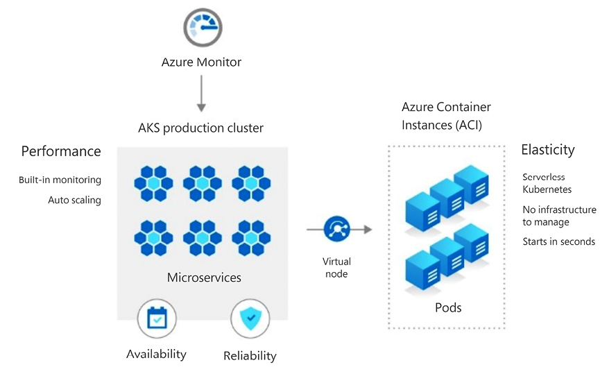
Figure 3.4: AKS and ACI

In this section, we looked at various factors that impact your decision regarding cluster capacity as well as cloud-provider solutions that do the heavy lifting on your behalf. In the next section, we will see how far you can stress a single Kubernetes cluster.

Pushing the envelope with Kubernetes

In this section, we will see how the Kubernetes team pushes Kubernetes to its limit. The numbers are quite telling, but some of the tools and techniques, such as Kubemark, are ingenious, and you may even use them to test your clusters. Kubernetes is designed to support clusters with the following properties:

• Up to 110 pods per node
• Up to 5,000 nodes
• Up to 150,000 pods
• Up to 300,000 total containers

Those numbers are just guidelines and not hard limits. Clusters that host specialized workloads with specialized deployment and runtime patterns regarding new pods coming and going may support very different numbers.

At CERN, the OpenStack team achieved 2 million requests per second: http://superuser.openstack.org/articles/scaling-magnum-and-kubernetes-2-million-requests-per-second.

Mirantis conducted a performance and scaling test in their scaling lab where they deployed 5,000 Kubernetes nodes (in VMs) on 500 physical servers.

OpenAI scaled their machine learning Kubernetes cluster to 2,500 nodes on Azure and learned some valuable lessons such as minding the query load of logging agents and storing events in a separate etcd cluster: https://openai.com/research/scaling-kubernetes-to-2500-nodes.

There are many more interesting use cases here: https://www.cncf.io/projects/case-studies.

By the end of this section, you’ll appreciate the effort and creativeness that goes into improving Kubernetes on a large scale, you will know how far you can push a single Kubernetes cluster and what performance to expect, and you’ll get an inside look at some tools and techniques that can help you evaluate the performance of your own Kubernetes clusters.

Improving the performance and scalability of Kubernetes

The Kubernetes team focused heavily on performance and scalability in Kubernetes 1.6. When Kubernetes 1.2 was released, it supported clusters of up to 1,000 nodes within the Kubernetes service-level objectives. Kubernetes 1.3 doubled the number to 2,000 nodes, and Kubernetes 1.6 brought it to a staggering 5,000 nodes per cluster. 5,000 nodes can carry you very far, especially if you use large nodes. But, when you run large nodes, you need to pay attention to pods per node guideline too. Note that cloud providers still recommend up to 1,000 nodes per cluster.

We will get into the numbers later, but first, let’s look under the hood and see how Kubernetes achieved these impressive improvements.

Caching reads in the API server

Kubernetes keeps the state of the system in etcd, which is very reliable, though not super-fast (although etcd 3 delivered massive improvement specifically to enable larger Kubernetes clusters). The various Kubernetes components operate on snapshots of that state and don’t rely on real-time updates. That fact allows the trading of some latency for throughput. All the snapshots used to be updated by etcd watches. Now, the API server has an in-memory read cache that is used for updating state snapshots. The in-memory read cache is updated by etcd watches. These schemes significantly reduce the load on etcd and increase the overall throughput of the API server.

The pod lifecycle event generator

Increasing the number of nodes in a cluster is key for horizontal scalability, but pod density is crucial too. Pod density is the number of pods that the kubelet can manage efficiently on one node. If pod density is low, then you can’t run too many pods on one node. That means that you might not benefit from more powerful nodes (more CPU and memory per node) because the kubelet will not be able to manage more pods. The other alternative is to force the developers to compromise their design and create coarse-grained pods that do more work per pod. Ideally, Kubernetes should not force your hand when it comes to pod granularity. The Kubernetes team understands this very well and invested a lot of work in improving pod density.

In Kubernetes 1.1, the official (tested and advertised) number was 30 pods per node. I actually ran 40 pods per node on Kubernetes 1.1, but I paid for it in excessive kubelet overhead that stole CPU from the worker pods. In Kubernetes 1.2, the number jumped to 100 pods per node. The kubelet used to poll the container runtime constantly for each pod in its own goroutine. That put a lot of pressure on the container runtime that, during peaks to performance, has reliability issues, in particular CPU utilization. The solution was the Pod Lifecycle Event Generator (PLEG). The way the PLEG works is that it lists the state of all the pods and containers and compares it to the previous state. This is done once for all the pods and containers. Then, by comparing the state to the previous state, the PLEG knows which pods need to sync again and invokes only those pods. That change resulted in a significant four-times-lower CPU usage by the kubelet and the container runtime. It also reduced the polling period, which improves responsiveness.

The following diagram shows the CPU utilization for 120 pods on Kubernetes 1.1 versus Kubernetes 1.2. You can see the 4X factor very clearly:

Figure 3.5: CPU utilization for 120 pods with Kube 1.1 and Kube 1.2

Serializing API objects with protocol buffers

The API server has a REST API. REST APIs typically use JSON as their serialization format, and the Kubernetes API server was no different. However, JSON serialization implies marshaling and unmarshaling JSON to native data structures. This is an expensive operation. In a large-scale Kubernetes cluster, a lot of components need to query or update the API server frequently. The cost of all that JSON parsing and composition adds up quickly. In Kubernetes 1.3, the Kubernetes team added an efficient protocol buffers serialization format. The JSON format is still there, but all internal communication between Kubernetes components uses the protocol buffers serialization format.

etcd3

Kubernetes switched from etcd2 to etcd3 in Kubernetes 1.6. This was a big deal. Scaling Kubernetes to 5,000 nodes wasn’t possible due to limitations of etcd2, especially related to the watch implementation. The scalability needs of Kubernetes drove many of the improvements of etcd3, as CoreOS used Kubernetes as a measuring stick. Some of the big ticket items are talked about here.

gRPC instead of REST

etcd2 has a REST API, and etcd3 has a gRPC API (and a REST API via gRPC gateway). The HTTP/2 protocol at the base of gRPC can use a single TCP connection for multiple streams of requests and responses.

Leases instead of TTLs

etcd2 uses Time to Live (TTL) per key as the mechanism to expire keys, while etcd3 uses leases with TTLs where multiple keys can share the same key. This significantly reduces keep-alive traffic.

Watch implementation

The watch implementation of etcd3 takes advantage of gRPC bidirectional streams and maintains a single TCP connection to send multiple events, which reduced the memory footprint by at least an order of magnitude.

State storage

With etcd3, Kubernetes started storing all the state as protocol buffers, which eliminated a lot of wasteful JSON serialization overhead.

Other optimizations

The Kubernetes team made many other optimizations such as:

• Optimizing the scheduler (which resulted in 5-10x higher scheduling throughput)
• Switching all controllers to a new recommended design using shared informers, which reduced resource consumption of controller-manager
• Optimizing individual operations in the API server (conversions, deep copies, and patch)
• Reducing memory allocation in the API server (which significantly impacts the latency of API calls)

Measuring the performance and scalability of Kubernetes

In order to improve performance and scalability, you need a sound idea of what you want to improve and how you’re going to measure the improvements. You must also make sure that you don’t violate basic properties and guarantees in the quest for improved performance and scalability. What I love about performance improvements is that they often buy you scalability improvements for free. For example, if a pod needs 50% of the CPU of a node to do its job and you improve performance so that the pod can do the same work using 33% CPU, then you can suddenly run three pods instead of two on that node, and you’ve improved the scalability of your cluster by 50% overall (or reduced your cost by 33%).

The Kubernetes SLOs

Kubernetes has service level objectives (SLOs). Those guarantees must be respected when trying to improve performance and scalability. Kubernetes has a one-second response time for API calls (99 percentile). That’s 1,000 milliseconds. It actually achieves an order of magnitude faster response times most of the time.

Measuring API responsiveness

The API has many different endpoints. There is no simple API responsiveness number. Each call has to be measured separately. In addition, due to the complexity and the distributed nature of the system, not to mention networking issues, there can be a lot of volatility in the results. A solid methodology is to break the API measurements into separate endpoints and then run a lot of tests over time and look at percentiles (which is standard practice).

It’s also important to use enough hardware to manage a large number of objects. The Kubernetes team used a 32-core VM with 120 GB for the master in this test.

The following diagram describes the 50th, 90th, and 99th percentile of various important API call latencies for Kubernetes 1.3. You can see that the 90th percentile is very low, below 20 milliseconds. Even the 99th percentile is less than 125 milliseconds for the DELETE pods operation and less than 100 milliseconds for all other operations:

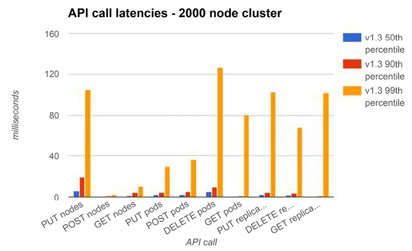
Figure 3.6: API call latencies

Another category of API calls is LIST operations. Those calls are more expansive because they need to collect a lot of information in a large cluster, compose the response, and send a potentially large response. This is where performance improvements such as the in-memory read cache and the protocol buffers serialization really shine. The response time is understandably greater than the single API calls, but it is still way below the SLO of one second (1,000 milliseconds):

Figure 3.7: LIST API call latencies

Measuring end-to-end pod startup time

One of the most important performance characteristics of a large dynamic cluster is end-to-end pod startup time. Kubernetes creates, destroys, and shuffles pods around all the time. You could say that the primary function of Kubernetes is to schedule pods. In the following diagram, you can see that pod startup time is less volatile than API calls. This makes sense since there is a lot of work that needs to be done, such as launching a new instance of a runtime, that doesn’t depend on cluster size. With Kubernetes 1.2 on a 1,000-node cluster, the 99th percentile end-to-end time to launch a pod was less than 3 seconds. With Kubernetes 1.3, the 99th percentile end-to-end time to launch a pod was a little over 2.5 seconds.

It’s remarkable that the time is very close, but a little better with Kubernetes 1.3, on a 2,000-node cluster versus a 1,000-node cluster:

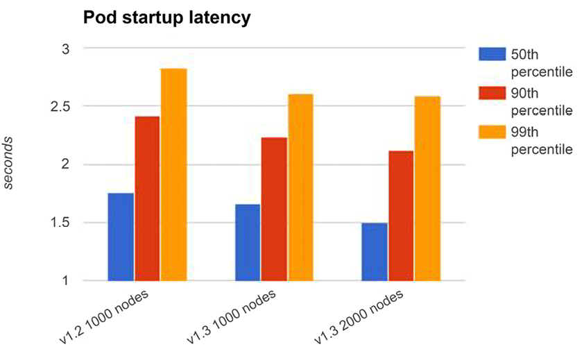
Figure 3.8: Pod startup latencies 1

Figure 3.9: Pod startup latencies 2

In this section, we looked at how far we can push Kubernetes and how clusters with a large number of nodes perform. In the next section, we will examine some of the creative ways the Kubernetes developers test Kubernetes at scale.

Testing Kubernetes at scale

Clusters with thousands of nodes are expensive. Even a project such as Kubernetes that enjoys the support of Google and other industry giants still needs to come up with reasonable ways to test without breaking the bank.

The Kubernetes team runs a full-fledged test on a real cluster at least once per release to collect real-world performance and scalability data. However, there is also a need for a lightweight and cheaper way to experiment with potential improvements and detect regressions. Enter Kubemark.

Introducing the Kubemark tool

Kubemark is a Kubernetes cluster that runs mock nodes called hollow nodes used for running lightweight benchmarks against large-scale (hollow) clusters. Some of the Kubernetes components that are available on a real node such as the kubelet are replaced with a hollow kubelet. The hollow kubelet fakes a lot of the functionality of a real kubelet. A hollow kubelet doesn’t actually start any containers, and it doesn’t mount any volumes. But from the Kubernetes point of view – the state stored in etcd – all those objects exist and you can query the API server. The hollow kubelet is actually the real kubelet with an injected mock Docker client that doesn’t do anything.

Another important hollow component is the hollow proxy, which mocks the kube-proxy component. It again uses the real kube-proxy code with a mock proxier interface that does nothing and avoids touching iptables.

Setting up a Kubemark cluster

A Kubemark cluster uses the power of Kubernetes. To set up a Kubemark cluster, perform the following steps:

1. Create a regular Kubernetes cluster where we can run N hollow nodes.
2. Create a dedicated VM to start all master components for the Kubemark cluster.
3. Schedule N hollow node pods on the base Kubernetes cluster. Those hollow nodes are configured to talk to the Kubemark API server running on the dedicated VM.
4. Create add-on pods by scheduling them on the base cluster and configuring them to talk to the Kubemark API server.

A full-fledged guide is available here:

https://github.com/kubernetes/community/blob/master/contributors/devel/sig-scalability/kubemark-guide.md

Comparing a Kubemark cluster to a real-world cluster

The performance of Kubemark clusters is mostly similar to the performance of real clusters. For the pod startup end-to-end latency, the difference is negligible. For the API responsiveness, the differences are greater, though generally less than a factor of two. However, trends are exactly the same: an improvement/regression on a real cluster is visible as a similar percentage drop/increase in metrics on Kubemark.

Summary

In this chapter, we looked at reliable and highly available large-scale Kubernetes clusters. This is arguably the sweet spot for Kubernetes. While it is useful to be able to orchestrate a small cluster running a few containers, it is not necessary, but at scale, you must have an orchestration solution in place that you can trust to scale with your system and provide the tools and the best practices to do that.

You now have a solid understanding of the concepts of reliability and high availability in distributed systems. You delved into the best practices for running reliable and highly available Kubernetes clusters. You explored the complex issues surrounding scaling Kubernetes clusters and measuring their performance. You can now make wise design choices regarding levels of reliability and availability, as well as their performance and cost.

In the next chapter, we will address the important topic of security in Kubernetes. We will also discuss the challenges of securing Kubernetes and the risks involved. We will learn all about namespaces, service accounts, admission control, authentication, authorization, and encryption.

Join us on Discord!

Read this book alongside other users, cloud experts, authors, and like-minded professionals.

Ask questions, provide solutions to other readers, chat with the authors via. Ask Me Anything sessions and much more.

Scan the QR code or visit the link to join the community now.

https://packt.link/cloudanddevops