
12
Harnessing Big Data with MongoDB
MongoDB is often used in conjunction with big data pipelines because of its performance, flexibility, and lack of rigorous data schemas. This chapter will explore the big data landscape, and how MongoDB fits alongside message queuing, data warehousing, and extract, transform, and load (ETL) pipelines.
We will also learn what the MongoDB Atlas Data Lake platform is and how to use this cloud data warehousing offering from MongoDB.
These are the topics that we will discuss in this chapter:
- What is big data?
- Big data use case with servers on-premises
- MongoDB Atlas Data Lake
Technical requirements
To follow along with the examples in this chapter, we need to install Apache Hadoop and Apache Kafka and connect to a MongoDB cluster such as the one that we created using MongoDB Atlas in the previous chapters. We need a trial account for MongoDB Atlas to use MongoDB Atlas Data Lake.
What is big data?
In the last 10 years, the number of people accessing and using the internet has grown from a little under 2 billion to 3.7 billion to 5.3 billion as of 2022. Around two-thirds of the global population is now online.
With the number of internet users increasing, and with networks evolving, more data is being added to existing datasets each year. In 2016, global internet traffic was 1.2 zettabytes (ZB) (which is 1.2 billion terabytes (TB)) and has grown to an expected 3.6 ZB in 2022.
This enormous amount of data that is generated every year means that it is imperative that databases and data stores, in general, can scale and process our data efficiently.
The term big data was first coined in the 1980s by John Mashey (http://static.usenix.org/event/usenix99/invited_talks/mashey.pdf), and mostly came into play in the past decade with the explosive growth of the internet. Big data typically refers to datasets that are too large and complex to be processed by traditional data processing systems, and so need some kind of specialized system architecture to be processed.
Big data’s defining characteristics are, in general, these:
- Volume
- Variety
- Velocity
- Veracity
- Variability
Variety and variability refer to the fact that our data comes in different forms and our datasets have internal inconsistencies. These need to be smoothed out by a data cleansing and normalization system before we can actually process our data.
Veracity refers to the uncertainty of the quality of data. Data quality may vary, with perfect data for some dates and missing datasets for others. This affects our data pipeline and how much we can invest in our data platforms since, even today, one out of three business leaders doesn’t completely trust the information they use to make business decisions.
Finally, velocity is probably the most important defining characteristic of big data (other than the obvious volume attribute), and it refers to the fact that big datasets not only have large volumes of data but also grow at an accelerated pace. This makes traditional storage using—for example—indexing a difficult task.
The big data landscape
Big data has evolved into a complex ecosystem affecting every sector of the economy. Going from hype to unrealistic expectations and back to reality, we now have big data systems implemented and deployed in most Fortune 1000 companies that deliver real value.
If we segmented the companies that participate in the big data landscape by industry, we would probably come up with the following sections:
- Infrastructure
- Analytics
- Applications-enterprise
- Applications-industry
- Cross-infrastructure analytics
- Data sources and application programming interfaces (APIs)
- Data resources
- Open source
From an engineering point of view, we are probably more concerned about the underlying technologies than their applications in different industry sectors.
Depending on our business domain, we may have data coming in from different sources, such as transactional databases, Internet of Things (IoT) sensors, application server logs, other websites via a web service API, or just plain web page content extraction, as illustrated in the following diagram:
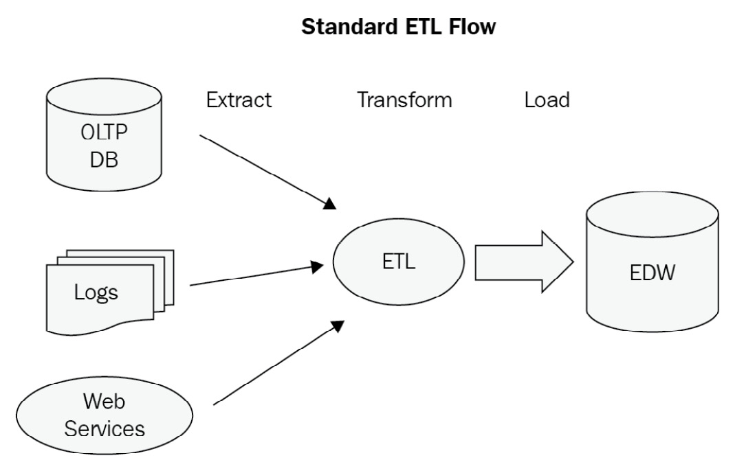
Figure 12.1: A sample ETL data flow
Message queuing systems
In most of the flows previously described, we have data being ETLed into an enterprise data warehouse (EDW). To extract and transform this data, we need a message queuing system to deal with spikes in traffic, endpoints being temporarily unavailable, and other issues that may affect the availability and scalability of this part of the system.
Message queues also provide decoupling between producers and consumers of messages. This allows for better scalability by partitioning our messages into different topics/queues.
Finally, using message queues, we can have location-agnostic services that don’t care where the message producers sit, which provides interoperability between different systems.
In the message queuing world, the most popular systems in production at the time of writing this book are RabbitMQ, ActiveMQ, and Kafka. We will provide a small overview of them before we dive into our use case to bring all of them together.
Apache ActiveMQ
Apache ActiveMQ is an open source message broker, written in Java, together with a full Java Message Service (JMS) client.
It is the most mature implementation out of the three that we examine here and has a long history of successful production deployments. Commercial support is offered by many companies, including Red Hat.
It is a fairly simple queuing system to set up and manage. It is based on the JMS client protocol and is the tool of choice for Java Enterprise Edition (EE) systems.
RabbitMQ
RabbitMQ, on the other hand, is written in Erlang and is based on Advanced Message Queuing Protocol (AMQP). AMQP is significantly more powerful and complicated than JMS, as it allows peer-to-peer messaging, request/reply, and publish/subscribe (pub/sub) models for one-to-one or one-to-many message consumption.
RabbitMQ has gained popularity in the past 5 years and is now the most searched-for queuing system.
RabbitMQ’s architecture is outlined as follows:
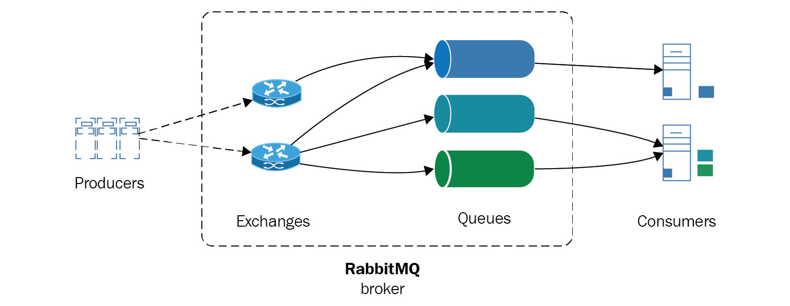
Figure 12.2: RabbitMQ architecture
Scaling in RabbitMQ systems is performed by creating a cluster of RabbitMQ servers. Clusters share data and state, which are replicated, but message queues are distinct per node. To achieve high availability (HA), we can also replicate queues in different nodes.
Apache Kafka
Kafka, on the other hand, is a queuing system that was first developed by LinkedIn for its own internal purposes. It is written in Scala and is designed from the ground up for horizontal scalability and the best performance possible.
Focusing on performance is a key differentiator for Apache Kafka, but it means that in order to achieve performance, we need to sacrifice something. Messages in Kafka don’t hold unique identifiers (UIDs) but are addressed by their offset in the log. Apache Kafka consumers are not tracked by the system; it is the responsibility of the application design to do so. Message ordering is implemented at the partition level, and it is the responsibility of the consumer to identify whether a message has been delivered already.
Semantics were introduced in version 0.11 and are part of the latest 1.0 release so that messages can now be both strictly ordered within a partition and always arrive exactly once for each consumer, as illustrated in the following diagram:
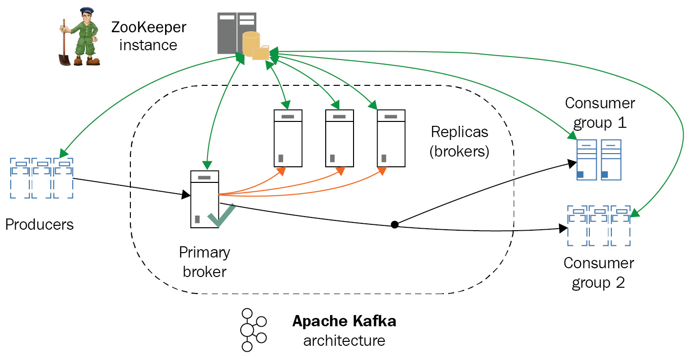
Figure 12.3: Apache Kafka architecture
The preceding diagram shows the overall Apache Kafka architecture. In the next section, we will learn about how to use MongoDB for data warehousing.
Data warehousing
Using a message queuing system is just the first step in our data pipeline design. At the other end of message queuing, we would typically have a data warehouse to process the vast amount of data that arrives. There are numerous options there, and it is not the main focus of this book to go over these or compare them. However, we will skim through two of the most widely used options from the Apache Software Foundation (ASF): Apache Hadoop and Apache Spark.
Apache Hadoop
The first, and probably still most widely used, framework for big data processing is Apache Hadoop. Its foundation is HDFS. Developed at Yahoo! in the 2000s, it originally served as an open source alternative to Google File System (GFS), a distributed filesystem that was serving Google’s needs for distributed storage of its search index.
Hadoop also implemented a MapReduce alternative to Google’s proprietary system, Hadoop MapReduce. Together with HDFS, they constitute a framework for distributed storage and computations. Written in Java, with bindings for most programming languages and many projects that provide abstracted and simple functionality, and sometimes based on Structured Query Language (SQL) querying, it is a system that can reliably be used to store and process TB, or even petabytes (PB), of data.
In later versions, Hadoop became more modularized by introducing Yet Another Resource Negotiator (YARN), which provides the abstraction for applications to be developed on top of Hadoop. This has enabled several applications to be deployed on top of Hadoop, such as Storm, Tez, Open MPI, Giraph, and, of course, Apache Spark, as we will see in the following sections.
Hadoop MapReduce is a batch-oriented system, meaning that it relies on processing data in batches, and is not designed for real-time use cases.
Apache Spark
Apache Spark is a cluster-computing framework from the University of California, Berkeley’s AMPLab. Spark is not a substitute for the complete Hadoop ecosystem, but mostly for the MapReduce aspect of a Hadoop cluster. Whereas Hadoop MapReduce uses on-disk batch operations to process data, Spark uses both in-memory and on-disk operations. As expected, it is faster with datasets that fit in memory. This is why it is more useful for real-time streaming applications, but it can also be used with ease for datasets that don’t fit in memory.
Apache Spark can run on top of HDFS using YARN or in standalone mode, as shown in the following diagram:
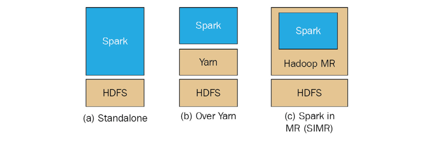
Figure 12.4: Apache Spark over HDFS
This means that in some cases (such as the one that we will use in our following use case), we can completely ditch Hadoop for Spark if our problem is really well defined and constrained within Spark’s capabilities.
Spark can be up to 100 times faster than Hadoop MapReduce for in-memory operations. Spark offers user-friendly APIs for Scala (its native language), Java, Python, and Spark SQL (a variation of the SQL-92 specification). Both Spark and MapReduce are resilient to failure. Spark uses resilient distributed datasets (RDDs) that are distributed across the whole cluster.
As we can see from the overall Spark architecture, as follows, we can have several different modules of Spark working together for different needs, from SQL querying to streaming and machine learning (ML) libraries.
Comparing Spark with Hadoop MapReduce
The Hadoop MapReduce framework is more commonly compared to Apache Spark, a newer technology that aims to solve problems in a similar problem space. Some of their most important attributes are summarized in the following table:
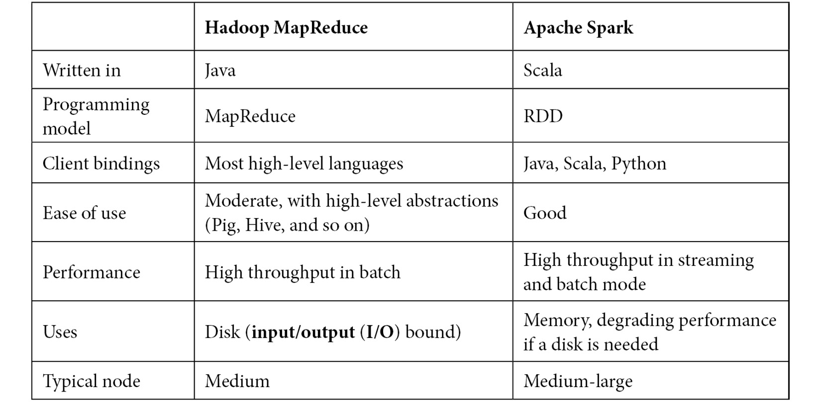
Table 12.1: Apache Spark versus Hadoop MapReduce framework comparison
As we can see from the preceding comparison, there are pros and cons for both technologies. Spark arguably has better performance, especially in problems that use fewer nodes. On the other hand, Hadoop is a mature framework with excellent tooling on top of it to cover almost every use case.
MongoDB as a data warehouse
Apache Hadoop is often described as the 800-pound gorilla in the room of big data frameworks. Apache Spark, on the other hand, is more like a 200-pound cheetah for its speed, agility, and performance characteristics, which allow it to work well in a subset of the problems that Hadoop aims to solve.
MongoDB, on the other hand, can be described as the MySQL equivalent in the NoSQL world, because of its adoption and ease of use. MongoDB also offers an aggregation framework, MapReduce capabilities, and horizontal scaling using sharding, which is essentially data partitioning at the database level. So, naturally, some people wonder why we don’t use MongoDB as our data warehouse to simplify our architecture.
This is a pretty compelling argument, and it may or may not be the case that it makes sense to use MongoDB as a data warehouse. The advantages of such a decision are set out here:
- Simpler architecture
- Less need for message queues, reducing latency in our system
The disadvantages are presented here:
- MongoDB’s MapReduce framework is not a replacement for Hadoop’s MapReduce. Even though they both follow the same philosophy, Hadoop can scale to accommodate larger workloads.
- Scaling MongoDB’s document storage using sharding will lead to hitting a wall at some point. Whereas Yahoo! has reported using 42,000 servers in its largest Hadoop cluster, the largest MongoDB commercial deployments stand at 5 billion (Craigslist), compared to 600 nodes and PB of data for Baidu, the internet giant dominating, among others, the Chinese internet search market.
There is more than an order of magnitude (OOM) of difference in terms of scaling.
MongoDB is mainly designed around being a real-time querying database based on stored data on disk, whereas MapReduce is designed around using batches, and Spark is designed around using streams of data.
Big data use case with servers on-premises
Putting all of this into action, we will develop a fully working system using a data source, a Kafka message broker, an Apache Spark cluster on top of HDFS feeding a Hive table, and a MongoDB database. Our Kafka message broker will ingest data from an API, streaming market data for a Monero (XMR)/Bitcoin (BTC) currency pair. This data will be passed on to an Apache Spark algorithm on HDFS to calculate the price for the next ticker timestamp, based on the following factors:
- The corpus of historical prices already stored on HDFS
- The streaming market data arriving from the API
This predicted price will then be stored in MongoDB using the MongoDB Connector for Hadoop. MongoDB will also receive data straight from the Kafka message broker, storing it in a special collection with the document expiration date set to 1 minute. This collection will hold the latest orders, with the goal of being used by our system to buy or sell, using the signal coming from the Spark ML system.
So, for example, if the price is currently 10 and we have a bid for 9.5, but we expect the price to go down at the next market tick, then the system would wait. If we expect the price to go up in the next market tick, then the system would increase the bid price to 10.01 to match the price in the next ticker.
Similarly, if the price is 10 and we bid for 10.5, but expect the price to go down, we would adjust our bid to 9.99 to make sure we don’t overpay for it. But if the price is expected to go up, we would immediately buy to make a profit at the next market tick.
Schematically, our architecture looks like this:
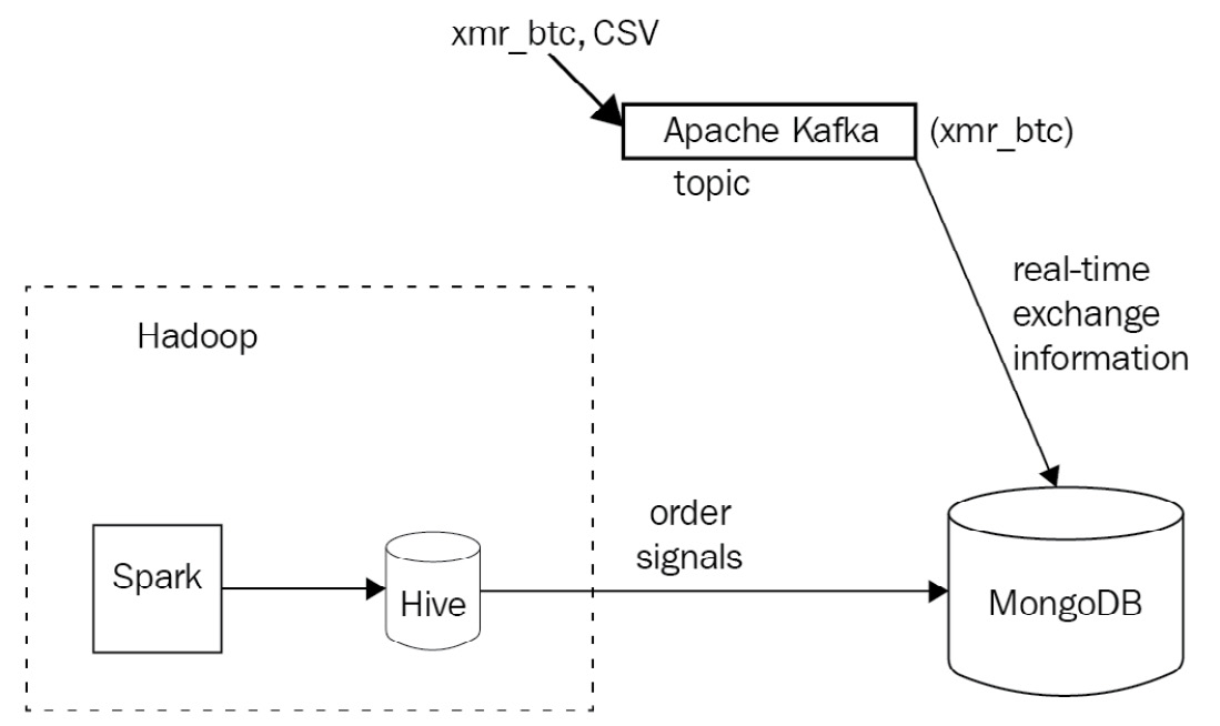
Figure 12.5: Sample use case Apache Kafka architecture
The API is simulated by posting JavaScript Object Notation (JSON) messages to a Kafka topic named xmr_btc. On the other end, we have a Kafka consumer importing real-time data to MongoDB.
We also have another Kafka consumer importing data to Hadoop to be picked up by our algorithms, which send recommendation data (signals) to a Hive table. Finally, we export data from the Hive table into MongoDB.
Setting up Kafka
The first step in setting up the environment for our big data use case is to establish a Kafka node. Kafka is essentially a first-in, first-out (FIFO) queue, so we will use the simplest single node (broker) setup. Kafka organizes data using topics, producers, consumers, and brokers.
The important Kafka terminologies are noted here:
- A broker is essentially a node
- A producer is a process that writes data to the message queue
- A consumer is a process that reads data from the message queue
- A topic is a specific queue that we write to and read data from
A Kafka topic is further subdivided into a number of partitions. We can split data from a particular topic into multiple brokers (nodes), both when we write to the topic and also when we read our data at the other end of the queue.
After installing Kafka on our local machine, or any cloud provider of our choice (there are excellent tutorials for Elastic Compute Cloud (EC2) to be found just a search away), we can create a topic using this single command:
$ kafka-topics --create --zookeeper localhost:2181 --replication-factor 1 --partitions 1 --topic xmr-btc
Created topic "xmr-btc".
This will create a new topic called xmr-btc.
Deleting the topic is similar to creating one, by using this command:
$ kafka-topics --delete --zookeeper localhost:2181 --topic xmr-btc
We can then get a list of all topics by issuing the following command:
$ kafka-topics --list --zookeeper localhost:2181
xmr-btc
We can then create a command-line producer for our topic, just to test that we can send messages to the queue, like this:
$ kafka-console-producer --broker-list localhost:9092 --topic xmr-btc
Data on every line will be sent as a string-encoded message to our topic, and we can end the process by sending a SIGINT signal (typically Ctrl + C).
Afterward, we can view messages that are waiting in our queue by spinning up a consumer, as follows:
$ kafka-console-consumer --zookeeper localhost:2181 --topic xmr-btc --from-beginning
This consumer will read all messages in our xmr-btc topic, starting from the beginning of history. This is useful for our test purposes, but we will change this configuration in real-world applications.
Note
You will keep seeing zookeeper, in addition to kafka, mentioned in the commands. Apache ZooKeeper comes together with Apache Kafka and is a centralized service that is used internally by Kafka for maintaining configuration information, naming, providing distributed synchronization, and providing group services.
Now that we have set up our broker, we can use the code at https://github.com/PacktPublishing/Mastering-MongoDB-6.x/tree/main/chapter_12 to start reading (consuming) and writing (producing) messages to the queue. For our purposes, we are using the ruby-kafka gem, developed by Zendesk.
For simplicity, we are using a single class to read from a file stored on disk and to write to our Kafka queue.
Our produce method will be used to write messages to Kafka, as follows:
def produce
options = { converters: :numeric, headers: true }CSV.foreach('xmr_btc.csv', options) do |row|json_line = JSON.generate(row.to_hash)
@kafka.deliver_message(json_line, topic: 'xmr-btc')
end
end
Our consume method will read messages from Kafka, as follows:
def consume
consumer = @kafka.consumer(group_id: 'xmr-consumers')
consumer.subscribe('xmr-btc', start_from_beginning: true)trap('TERM') { consumer.stop }consumer.each_message(automatically_mark_as_processed: false) do |message|
puts message.value
if valid_json?(message.value)
MongoExchangeClient.new.insert(message.value)
consumer.mark_message_as_processed(message)
end
end
consumer.stop
end
Note
Notice that we are using the consumer group API feature (added in Kafka 0.9) to get multiple consumers to access a single topic by assigning each partition to a single consumer. In the event of a consumer failure, its partitions will be reallocated to the remaining members of the group.
The next step is to write these messages to MongoDB, as follows:
- First, we create a collection so that our documents expire after 1 minute. Enter the following code in the mongo shell:
> use exchange_data
> db.xmr_btc.createIndex( { "createdAt": 1 }, { expireAfterSeconds: 60 })
{
"createdCollectionAutomatically" : true,
"numIndexesBefore" : 1,
"numIndexesAfter" : 2,
"ok" : 1
}
This way, we create a new database called exchange_data with a new collection called xmr_btc that has auto-expiration after 1 minute. For MongoDB to auto-expire documents, we need to provide a field with a datetime value to compare its value against the current server time. In our case, this is the createdAt field.
- For our use case, we will use the low-level MongoDB Ruby driver. The code for MongoExchangeClient is shown here:
class MongoExchangeClient
def initialize
@collection = Mongo::Client.new([ '127.0.0.1:27017' ], database: :exchange_data).database[:xmr_btc]
end
def insert(document)
document = JSON.parse(document)
document['createdAt'] = Time.now
@collection.insert_one(document)
end
end
This client connects to our local database, sets the createdAt field for the time-to-live (TTL) document expiration, and saves the message to our collection.
With this set up, we can write messages to Kafka, read them at the other end of the queue, and write them into our MongoDB collection.
Setting up Hadoop
We can install Hadoop and use a single node for the use case in this chapter using the instructions from Apache Hadoop’s website at https://hadoop.apache.org/docs/stable/hadoop-project-dist/hadoop-common/SingleCluster.html.
After following these steps, we can browse the HDFS files in our local machine at http://localhost:50070/explorer.html#/. Assuming that our signals data is written in HDFS under the /user/<username>/signals directory, we will use the MongoDB Connector for Hadoop to export and import it into MongoDB.
The MongoDB Connector for Hadoop is the officially supported library, allowing MongoDB data files or MongoDB backup files in Binary JSON (BSON) to be used as the source or destination for Hadoop MapReduce tasks.
This means that we can also easily export to, and import data from, MongoDB when we are using higher-level Hadoop ecosystem tools such as Pig (a procedural high-level language), Hive (a SQL-like high-level language), and Spark (a cluster-computing framework).
Steps for Hadoop setup
The different steps to set up Hadoop are set out here:
- Download the Java ARchive (JAR) file from the Maven repository at https://repo1.maven.org/maven2/org/mongodb/mongo-hadoop/mongo-hadoop-core/2.0.2/.
- Download mongo-java-driver from https://oss.sonatype.org/content/repositories/releases/org/mongodb/mongodb-driver/3.5.0/.
- Create a directory (in our case, named mongo_lib) and copy these two JARs in there with the following command:
export HADOOP_CLASSPATH=$HADOOP_CLASSPATH:<path_to_directory>/mongo_lib/
Alternatively, we can copy these JARs under the share/hadoop/common/ directory. As these JARs will need to be available in every node, for clustered deployment, it’s easier to use Hadoop’s DistributedCache to distribute the JARs to all nodes.
- The next step is to install Hive from https://hive.apache.org/downloads.html. For this example, we used a MySQL server for Hive’s metastore data. This can be a local MySQL server for development, but it is recommended that you use a remote server for production environments.
- Once we have Hive set up, we just run the following command:
> hive
- Then, we add the three JARs (mongo-hadoop-core, mongo-hadoop-driver, and mongo-hadoop-hive) that we downloaded earlier, as follows:
hive> add jar /Users/dituser/code/hadoop-2.8.1/mongo-hadoop-core-2.0.2.jar;
Added [/Users/dituser/code/hadoop-2.8.1/mongo-hadoop-core-2.0.2.jar] to class path
Added resources: [/Users/dituser/code/hadoop-2.8.1/mongo-hadoop-core-2.0.2.jar]
hive> add jar /Users/dituser/code/hadoop-2.8.1/mongodb-driver-3.5.0.jar;
Added [/Users/dituser/code/hadoop-2.8.1/mongodb-driver-3.5.0.jar] to class path
Added resources: [/Users/dituser/code/hadoop-2.8.1/mongodb-driver-3.5.0.jar]
hive> add jar /Users/dituser/code/hadoop-2.8.1/mongo-hadoop-hive-2.0.2.jar;
Added [/Users/dituser/code/hadoop-2.8.1/mongo-hadoop-hive-2.0.2.jar] to class path
Added resources: [/Users/dituser/code/hadoop-2.8.1/mongo-hadoop-hive-2.0.2.jar]
hive>
And then, we assume our data is in the table exchanges shown here:
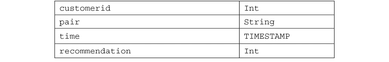
Table 12.2: Data types
Note
We can also use Gradle or Maven to download the JARs in our local project. If we only need MapReduce, then we just download the mongo-hadoop-core JAR. For Pig, Hive, Streaming, and so on, we must download the appropriate JARs from https://repo1.maven.org/maven2/org/mongodb/mongo-hadoop/.
Some useful Hive commands include the following: show databases; and create table exchanges(customerid int, pair String, time TIMESTAMP, recommendation int);.
- Now that we are all set, we can create a MongoDB collection backed by our local Hive data, as follows:
hive> create external table exchanges_mongo (objectid STRING, customerid INT,pair STRING,time STRING, recommendation INT) STORED BY 'com.mongodb.hadoop.hive.MongoStorageHandler' WITH SERDEPROPERTIES('mongo.columns.mapping'='{"objectid":"_id","customerid":"customerid","pair":"pair","time":"Timestamp", "recommendation":"recommendation"}') tblproperties('mongo.uri'='mongodb://localhost:27017/exchange_data.xmr_btc');
- Finally, we can copy all data from the exchanges Hive table into MongoDB, as follows:
hive> Insert into table exchanges_mongo select * from exchanges;
This way, we have established a pipeline between Hadoop and MongoDB using Hive, without any external server.
Using a Hadoop-to-MongoDB pipeline
An alternative to using the MongoDB Connector for Hadoop is to use the programming language of our choice to export data from Hadoop, and then write into MongoDB using the low-level driver or an object document mapper (ODM), as described in previous chapters.
For example, in Ruby, there are a few options, as follows:
- WebHDFS on GitHub, which uses the WebHDFS or the HttpFS Hadoop API to fetch data from HDFS
- System calls, using the Hadoop command-line tool and Ruby’s system() call
Whereas in Python, we can use the following:
- HdfsCLI, which uses the WebHDFS or the HttpFS Hadoop API
- libhdfs, which uses a Java Native Interface (JNI)-based native C wrapped around the HDFS Java client
All of these options require an intermediate server between our Hadoop infrastructure and our MongoDB server, but, on the other hand, allow for more flexibility in the ETL process of exporting/importing data.
Setting up a Spark connection to MongoDB
MongoDB also offers a tool to directly query Spark clusters and export data to MongoDB. Spark is a cluster computing framework that typically runs as a YARN module in Hadoop, but can also run independently on top of other filesystems.
The MongoDB Spark Connector can read and write to MongoDB collections from Spark using Java, Scala, Python, and R. It can also use aggregation and run SQL queries on MongoDB data after creating a temporary view for the dataset backed by Spark.
Using Scala, we can also use Spark Streaming, the Spark framework for data-streaming applications built on top of Apache Spark.
In the next section, we will discuss how to use data warehousing in the cloud, using the MongoDB Atlas Data Lake service.
MongoDB Atlas Data Lake
A data lake is a centralized repository that can be used to store, query, and transform heterogeneous structured and unstructured data. As the name implies, it acts as a lake of data.
MongoDB Data Lake (https://www.mongodb.com/atlas/data-lake) is a service offered by MongoDB that can help us process datasets across multiple MongoDB Atlas clusters and Amazon Web Services (AWS) Simple Storage Service (S3) buckets.
A data lake can query data in multiple formats such as JSON, BSON, comma-separated values (CSV), tab-separated values (TSV), Avro, Optimized Row Columnar (ORC), and Parquet. We can query the datasets using any driver, graphical user interface (GUI) tools such as MongoDB Compass, or the MongoDB shell using the standard MongoDB Query Language (MQL).
We can use x509 or SCRAM-SHA authentication methods. MongoDB Data Lake does not support Lightweight Directory Access Protocol (LDAP).
A data lake can be used for a variety of big data use cases, including but not limited to the following:
- Querying data across multiple MongoDB Atlas clusters to generate business insights that were previously uncovered.
- Converting MongoDB data into one of the supported formats—for example, Parquet or Avro or CSV. This could be part of an ETL process to extract data from a MongoDB Atlas cluster into another system for reporting, ML, or other reasons.
- Ingest data into our MongoDB Atlas cluster from an S3 bucket. This could again be part of an ETL process.
- Process and store aggregations performed against MongoDB Atlas or S3-hosted data.
We need to grant read-only or read-write access to the S3 buckets that we want to use with MongoDB Data Lake. Atlas will use existing role-based access control (RBAC) to access the MongoDB clusters.
MongoDB Atlas Data Lake is the recommended approach for cloud-based big data systems, offering features and support by MongoDB.
Summary
In this chapter, we learned about the big data landscape and how MongoDB compares with, and fares against, message-queuing systems and data warehousing technologies. Using a big data use case, we learned how to integrate MongoDB with Kafka and Hadoop from a practical perspective. Finally, we learned about data lakes and how we can use them to store and process data from different data sources such as MongoDB Atlas and Amazon S3 buckets.
In the next chapter, we will turn to replication and cluster operations, and discuss replica sets, the internals of elections, and the setup and administration of our MongoDB cluster.
Further reading
You can refer to the following references for further information:
- Internet adoption estimates: https://www.cisco.com/c/en/us/solutions/collateral/service-provider/visual-networking-index-vni/vni-hyperconnectivity-wp.html
- Big data companies landscape (2017): http://mattturck.com/wp-content/uploads/2017/05/Matt-Turck-FirstMark-2017-Big-Data-Landscape.png
- Message queuing explained: https://www.cloudamqp.com/blog/2014-12-03-what-is-message-queuing.html
- JMS and AMQP message queuing systems: https://www.linkedin.com/pulse/jms-vs-amqp-eran-shaham
- Apache Kafka and RabbitMQ: https://www.cloudamqp.com/blog/2017-01-09-apachekafka-vs-rabbitmq.html
- MapReduce Google paper: https://static.googleusercontent.com/media/research.google.com/en//archive/mapreduce-osdi04.pdf
- Apache Hadoop architecture: https://en.wikipedia.org/wiki/Apache_Hadoop#Architecture
- YARN and MapReduce 2: https://www.slideshare.net/cloudera/introduction-to-yarn-and-mapreduce-2?next_slideshow=1
- MongoDB at Craigslist (2011): https://www.mongodb.com/blog/post/mongodb-live-at-craigslist
- MongoDB at Baidu (2016): https://www.mongodb.com/blog/post/mongodb-at-baidu-powering-100-apps-across-600-nodes-at-pb-scale
- Hadoop and Spark: http://www.datamation.com/data-center/hadoop-vs.-spark-the-new-age-of-big-data.html
- MongoDB as a Data Warehouse: https://www.mongodb.com/mongodb-data-warehouse-time-series-and-device-history-data-medtronic-transcript
- Hadoop and Apache Spark:
https://iamsoftwareengineer.wordpress.com/2015/12/15/hadoop-vs-spark/?iframe=true&theme_preview=true
- Apache Kafka: https://www.infoq.com/articles/apache-kafka
- Apache Kafka exactly-once message semantics: https://medium.com/@jaykreps/exactly-once-support-in-apache-kafka-55e1fdd0a35f
- Apache Kafka and RabbitMQ: https://www.slideshare.net/sbaltagi/apache-kafka-vs-rabbitmq-fit-for-purpose-decision-tree
- Kafka Ruby library: https://github.com/zendesk/ruby-kafka
- Apache Hadoop on Mac OS X tutorial: http://zhongyaonan.com/hadoop-tutorial/setting-up-hadoop-2-6-on-mac-osx-yosemite.html
- API and command-line interface (CLI) for HDFS: https://github.com/mtth/hdfs
- Python HDFS library: http://wesmckinney.com/blog/python-hdfs-interfaces/
- Kafka in a Nutshell: https://sookocheff.com/post/kafka/kafka-in-a-nutshell/
- Apache Spark and Python using MLlib: https://www.codementor.io/jadianes/spark-mllib-logistic-regression-du107neto
- Apache Spark and Ruby: http://ondra-m.github.io/ruby-spark/
- Apache Spark introduction: https://www.infoq.com/articles/apache-spark-introduction
- Apache Spark Stanford paper: https://cs.stanford.edu/~matei/papers/2010/hotcloud_spark.pdf