
Guided Learning Unit 1 Simple ideas of crystallography
Introduction and synopsis
Though they lacked the means to prove it, the ancient Greeks suspected that solids were made of discrete atoms that were packed in a regular, orderly way to give crystals. Today, with the 21st century techniques of X-ray and electron diffraction and lattice-resolution microscopy available to us, we know that all solids are indeed made of atoms, and that most (but not all) are crystalline. The common engineering metals and ceramics are made of many small crystals, or grains, stuck together at grain boundaries to make polycrystalline aggregates. The properties of the material—its strength, stiffness, toughness, conductivity and so forth—are strongly influenced by the underlying crystallinity. So it is important to be able to describe it.
Crystallography is a language for describing the 3-dimensional arrangement of atoms or molecules in crystals. Simple crystalline and non-crystalline structures were introduced earlier in the book. Here we go a little further, exploring a wider range of structures, interstitial space (important in understanding the hardness of steel), and ways of describing planes and directions in crystals (crucial in the production of turbine blades and in the manufacture of microchips).
Exercises are provided in Parts 1–4, so do these as you go along; solutions are provided at the end of the unit.
PART 1: Crystal structures
Three-dimensional crystal lattices may be characterised by the repeating geometry of the atomic arrangement they contain, particularly their degree of symmetry. In fact it may be shown that there are 14 distinguishable three-dimensional lattices. If you are a crystallographer you need to know about all of them1. But engineering materials, for the most part, have simple structures. We shall concentrate on these.
The great majority of the 92 stable elements are metallic, and of these, the majority (68 in all) have one of the three simple structures introduced in Chapter 4: face-centred cubic (FCC), body-centred cubic (BCC) and hexagonal close packed (HCP or CPH). We start by revisiting them briefly.
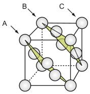
The face-centred cubic (FCC) structure
The FCC structure is described by a cubic unit cell with one atom at each corner and one at the centre of each face. Atoms touch along the diagonals of the cube faces. From a packing viewpoint, it consists of close-packed planes stacked in an ABCABC … sequence (Figure GL1.1).
Among the metallic elements, 17 have the FCC structure. Engineering materials with this structure include the following.
| Material | Typical uses |
|---|---|
| Aluminum and its alloys | Airframes, space frames and bodies of trains, trucks, cars, drink cans |
| Nickel and its alloys | Turbine blades and disks |
| Copper and α-brass | Conductors, bearings |
| Lead | Batteries, roofing, cladding of buildings |
| Austenitic stainless steels | Stainless cookware, chemical and nuclear engineering, cryogenic engineering |
| Silver, gold, platinum | Jewelry, coinage, electrical contacts |
FCC metals have the following characteristics:
- They are very ductile when pure, work hardening rapidly but softening again when annealed, allowing them to be rolled, forged, drawn or otherwise shaped by deformation processing.
- They are generally tough, resistant to crack propagation (as measured by their fracture toughness, K1c).
- They retain their ductility and toughness to absolute zero, something very few other structures allow.
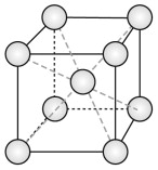
The body-centred cubic (BCC) structure
The BCC structure is described by a cubic unit cell with one atom at each corner and one in the middle of the cube (Figure GL1.2). The atoms touch along the internal diagonal of the cube.
Of the metallic elements, 21 have this structure (most are rare earths). They include the following.
| Material | Typical uses |
|---|---|
| Iron, mild steel | The most important metal of engineering: construction, cars, cans and more |
| Carbon steels, low alloy steels | Engine parts, tools, pipelines, power generation |
| Tungsten | Lamp filaments |
| Chromium | Electroplated coatings |
BCC metals have the following characteristics:
- They are ductile, particularly when hot, allowing them to be rolled, forged, drawn or otherwise shaped by deformation processing.
- They are generally tough, resistant to crack propagation (as measured by their fracture toughness, K1c) at and above room temperature.
- They become brittle at low temperatures. The change happens at the ‘ductile-brittle transition temperature’, limiting their use below this.
- Their strength depends on temperature, even at low temperatures.
- They can generally be hardened with interstitial solutes.
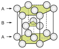
The close-packed hexagonal (HCP) structure
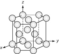
The HCP structure is usually described by a hexagonal unit cell with an atom at each corner, one at the centre of the hexagonal faces and three in the middle. From a packing viewpoint, it consists of close-packed planes stacked in an ABAB … sequence (Figure GL1.3).
Of the metallic elements, 30 have this structure. They include the following:
| Material | Typical uses |
|---|---|
| Zinc | Die-castings, plating |
| Magnesium | Lightweight structures |
| Titanium, its alloys | Light, strong components for airframes and engines, biomedical and chemical engineering |
| Cobalt | High temperature superalloys, bone-replacement implants |
| Beryllium | The lightest of the light metals; its use is limited by expense and potential toxicity |
HCP metals have the following characteristics.
- They are ductile, allowing them to be forged, rolled and drawn, but in a more limited way than FCC metals.
- Their structure makes them more anisotropic than FCC or BCC metals.
Exercises
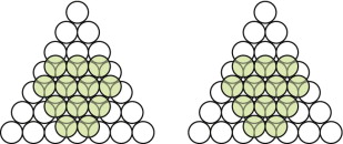
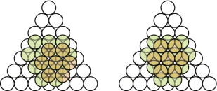
- E.1 Copper has an FCC structure. Draw the third layer on Figure GL1.4, below left, to make it.
- E.2 Magnesium has an HCP structure. Draw the third layer on Figure GL1.4, above right, to create this structure.
- E.3
- (a) How many atoms are contained within the FCC unit cell? (Hint: consider how many adjoining cells ‘share’ each corner atom and face atom in the cell.)
- (b) Determine the atomic packing factor (the fractional volume occupied) for an FCC structure, assuming that the atoms behave as hard spheres. (Note that in FCC, atoms touch along the diagonals of the face of the unit cell.)
- (c) The atomic diameter of an atom of nickel is 0.2492 nm. Calculate the lattice constant (the edge-length of the unit cell) of FCC nickel.
- (d) The atomic weight of nickel is 58.71 kg/kmol. Calculate the density of nickel. (The number of atoms in 1 kmol is Avogadro’s number = 6.022 × 1026.)
- E.4 Follow the same procedures as in Exercise E.3 to answer the following:
- (a) Determine the atomic packing factor for BCC, and comment on the value compared with that for FCC. (Note that in BCC, atoms touch along the internal diagonal of the unit cell.)
- (b) The atomic diameter of BCC iron is 0.2482 nm. Calculate the lattice constant of iron.
- (c) The atomic weight of iron is 55.85 kg/kmol. Calculate the density of iron.
PART 2: Interstitial space
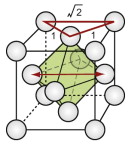
Interstitial space is the unit of space between the atoms of molecules. The FCC and HCP structures both contain interstitial space of two sorts: tetrahedral and octahedral. They are shown for the FCC structure in Figure GL1.5(a) and (b).
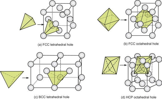
Figure GL1.5 (a) and (b) The two types of interstitial hole in the FCC structure, (c) the tetrahedral hole of the BCC structure and (d) the octahedral hole in the CPH structure.
The holes are important because foreign atoms, if small enough, can fit into them. For both structures, the tetrahedral hole can accommodate, without strain, a sphere with a radius of 0.22 of that of the host. The octahedral holes are larger: they can hold a sphere that is … but wait, that is Exercise E.5. The atoms of which crystals are made, in reality, are slightly squashy, so that foreign atoms that are larger than the holes can be squeezed into the interstitial space.
This is particularly important for carbon steel. Carbon steel is iron with carbon in some of the interstitial holes. Iron is BCC, and, like the FCC structure, it contains holes (Figure GL1.5(c)). They are tetrahedral. They can hold a sphere with a radius 0.29 times that of the host without distortion. Carbon goes into these holes, but, because it is too big, it distorts the structure. It is this distortion that gives carbon steels much of their strength.
The CPH structure, like the FCC, has both octahedral and tetrahedral interstitial holes. The larger of the two, the octahedral hole, is shown in Figure GL1.5(d). The holes have the same sizes as those in the FCC structure.
We shall encounter these interstitial holes in another context later: they provide a way of understanding the structures of many oxides, carbides and nitrides.
Now more Exercises, in the interstitial space before the next subsection.
Exercises
- E.5 Calculate the diameter of the largest sphere that will fit into the octahedral hole in the FCC structure. Take the diameter of the host-spheres to be unity.
- E.6 The HCP structure contains tetrahedral interstitial holes as well as octahedral ones. Identify a tetrahedral hole on the HCP lattice of Figure GL1.6.
PART 3: Describing planes
The properties of crystals depend on direction. The elastic modulus of hexagonal titanium (HCP), for example, is greater along the hexagonal axis than normal to it. This difference can be used in engineering design. In making titanium turbine blades, for example, it is helpful to align the hexagonal axis along a turbine blade to use the extra stiffness. Silicon (which also has a cubic structure) oxidises in a more uniform way on the cube faces than on other planes, so silicon ‘wafers’ are cut with their faces parallel to a cube face. For these and many other reasons, a way of describing planes and directions in crystals is needed. Miller indices provide it.
First, let’s describe planes. The Miller indices of a plane are the reciprocals of the intercepts the plane makes with the three axes that define the edges of the unit cell, reduced to the smallest integers.
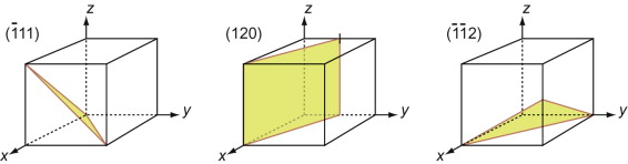
Figure GL1.7 illustrates how the Miller indices of a plane are found. Draw the plane in the unit cell so that it does not contain the origin—if it does, displace it along one axis until it doesn’t. Extend the plane until it intersects the axes. Measure the intercepts, in units of the cell edge-length, and take the reciprocals. (If the plane is parallel to an axis, its intercept is at infinity and the reciprocal is zero.) Reduce the result to the smallest set of integers by multiplying through to get rid of fractions or dividing to remove common factors. The six little sketches show, in order, the (100), the (110), the (111), the (211), the ![]() and the (112) planes; the
and the (112) planes; the ![]() means that the plane intercepts the y-axis at the point –1. Check that you get the same indices.
means that the plane intercepts the y-axis at the point –1. Check that you get the same indices.
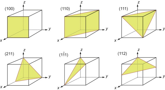
Figure GL1.7 The procedure for finding the Miller indices of a plane. The indices of four common planes are shown on the right.
The Miller indices of a plane are always written in round brackets: (111). But there are many planes of the 111-type; two are shown in Figure GL1.7. The complete family is described by putting the indices in curly brackets, thus:
Exercises
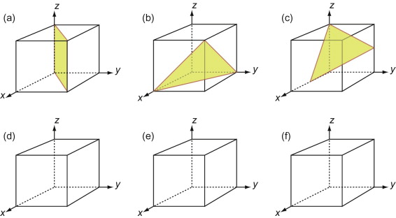
- E.7 What are the Miller indices of the planes shown in the six sketches of Figure GL1.8(a), (b) and (c)? (Remember that, to get the indices, the plane must not pass through the origin, and remember too to get rid of fractions or common factors.)
- E.8 When iron is cold it cleaves (fractures in a brittle way) on the (100) planes. What will be the angle between cleavage facets?
- E.9 Mark, on the cells of Figure GL1.8(d), (e) and (f), the following planes:
 , (120),
  .
.
PART 4: Describing directions
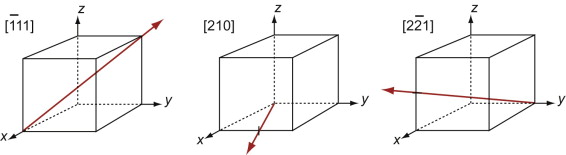
The Miller indices of a direction are the components of a vector (not reciprocals) that starts from the origin, along the direction, reduced to the smallest integer set.
Figure GL1.9 shows how to find the indices of a direction. Draw a line from the origin, parallel to the direction, extending it until it hits a cell edge or face. Read off the coordinates of the point of intersection. Get rid of any fraction or common factor by multiplying all the components by the same constant. The six sketches show the [010], the [011], the [111], the [021], the ![]() and the
and the ![]() directions. The
directions. The ![]() means that the y-coordinate of the intersection point is –1.
means that the y-coordinate of the intersection point is –1.
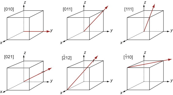
Figure GL1.9 Miller indices of directions. Always translate the direction so that it starts at the origin.
The Miller indices of a direction are always written in square brackets: [100]. As with planes, there are several directions of the 100-type. The complete family is described by putting the indices in angle-brackets, thus:
PART 5: Ceramic crystals
Technical ceramics give us the hardest, most refractory materials of engineering. Those of greatest economic importance include:
- Alumina, Al2O3 (spark plug insulators, substrates for microelectronic devices).
- Magnesia, MgO (refractories).
- Zirconia, ZrO2 (thermal barrier coatings, ceramic cutting tools).
- Uranium dioxide, UO2 (nuclear fuels).
- Silicon carbide, SiC (abrasives, cutting tools).
- Diamond, C (abrasives, cutting tools, dies, bearings).
The ceramic family also gives us many of the functional materials—those that are semiconductors, are ferromagnetic, show piezo-electric behaviour and so on. Their structures often look complicated, but when deconstructed, so to speak, a large number turn out to be comprehensible (and for good reasons) as atoms of one type arranged on a simple FCC, HCP or BCC lattice with the atoms of the second type (and sometimes a third) inserted into the interstices of the structure of the first.
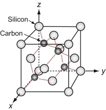
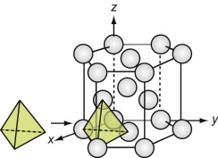
The diamond cubic (DC) structure
We start with the hardest ceramic of the lot—diamond—of major engineering importance for cutting tools, abrasives, polishes and scratch-resistant coatings, and at the same time as a valued gemstone for jewelry. Silicon and germanium, the foundation of semiconductor technology, have the same structure.
Figure GL1.11 shows the unit cell. Think of it as an FCC lattice with an additional atom in each of its tetrahedral interstices, labeled 1, 2, 3 and 4 in the figure. The tetrahedral hole is far too small to accommodate a full-sized atom, so the others are pushed farther apart, lowering the density. The cause is the 4-valent nature of the carbon, silicon and germanium atoms—they are happy only when each has 4 nearest neighbors, symmetrically placed around them. That is what this structure does.
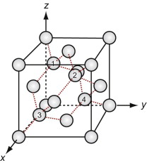
Silicon carbide, like diamond, is very hard, and it too is widely used for abrasives and cutting tools. The structures of the two materials are closely related. Carbon lies directly above silicon in the periodic table. Both have the same crystal structure and are chemically similar. So it comes as no surprise that a compound of the two with the formula SiC has a structure like that of diamond, with half the carbon atoms replaced by silicon, as in Figure GL1.12 (it is the atoms marked 1, 2, 3 and 4 of Figure GL1.11 that are replaced).
| Materials with the diamond-cubic structure | Comment |
|---|---|
| Carbon, as diamond | Cutting and grinding tools, jewelry |
| Silicon, germanium | Semiconductors |
| Silicon carbide | Abrasives, cutting tools |
Oxides with the Rocksalt (Halite) structure
These oxides all have the formula MO, where M is a metal ion. Oxygen ions are large, usually bigger than those of the metal. When this is so the oxygen packs in an FCC structure, the metal atoms occupy the octahedral holes in this lattice. The resulting structure is sketched in Figure GL1.13. This is known as the Rocksalt (or Halite) structure because it is that of sodium chloride, NaCl, with chlorine where the oxygens are and sodium where the magnesiums are in the figure.
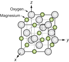
Sodium chloride (common salt) itself is a material of engineering importance. It has been used for road beds and buildings, there are plans to bury nuclear waste in rocksalt deposits; and large single crystals of rocksalt are used for the windows of high-powered lasers.
| Materials with the Rocksalt structure | Comment |
|---|---|
| Magnesia, MgO | A refractory, and ceramic with useful strength |
| Ferrous oxide, FeO | One of several oxides of iron |
| Nickel oxide, NiO | Ceramic superconductors |
| All alkali halides, including salt, NaCl | Feedstock for chemical industry, nuclear waste storage |
Oxides with the Corundum structure
A number of oxides have the formula M2O3, among them alumina, Al2O3. The oxygen ions, the larger of the two, are close packed in an HCP stacking. The M atoms occupy two-thirds of the octahedral holes in this lattice, one of which is shown for alumina, filled, in Figure GL1.14.
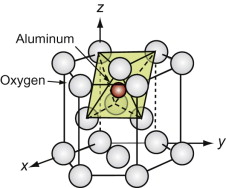
Figure GL1.14 The M atoms (here aluminum) of the Corundum structure lie in the octahedral holes of an HCP oxygen lattice.
| Materials with the Corundum structure | Comment |
|---|---|
| Alumina, Al2O3 | The most widely used technical ceramic |
| Iron oxide, Fe2O3 | The oxide from which iron is extracted |
| Chromium oxide, Cr2O3 | The oxide that gives chromium its protective coating |
| Titanium oxide, Ti2O3 | The oxide that gives titanium its protective coating |
Oxides with the Fluorite structure
The metal atoms in the important technical ceramic zirconium dioxide, ZrO2, and the nuclear fuel uranium dioxide, UO2, being far down in the periodic table, are large in size. Unlike the oxides described earlier, the M of the MO2 in these is larger than the O. In these it is the M atoms that form a close-packed FCC structure and it is the oxygens that fit into the tetrahedral interstices in it, as shown in Figure GL1.15.
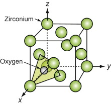
Figure GL1.15 The M atoms of fluorite-structured oxides pack in an FCC array, with oxygen in the tetrahedral interstices.
| Materials with the Fluorite structure | Comment |
|---|---|
| Zirconia, ZrO2 (slightly distorted fluorite) | The toughest high-temperature ceramic |
| Urania, UO2 | Nuclear fuel |
| Thoria, ThO2 | Nuclear fuel |
| Plutonia, Pu2O3 | A product of nuclear fuel reprocessing, a fuel in itself |
PART 6: Polymer crystals
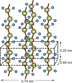
Many polymers crystallise. The long chains line up and pack to give an ordered, repeating structure, just like any other crystal. The low symmetry of the individual molecules means that the choice of lattice is limited. Figure GL1.16 is a typical example; it is polyethylene.
Few engineering polymers are completely crystalline, but many have as much as 90% crystallinity. Among those of engineering importance are:
| Material | Typical uses |
|---|---|
| Polyethylene, PE, 65–90% | Bags, tubes, bottles |
| Nylon, PA, 65% | High-quality parts, gears, catches |
| Polypropylene, PP, 75% | Mouldings, rope |
Answers to exercises
- E.1 The FCC packing of copper is shown in Figure GL1.17, left.
- E.2 The HCP packing in magnesium is shown in Figure GL1.17, right.
- E.3
- (a) Each corner atom is shared between 8 unit cells, and each face atom is shared between 2. There are 8 corners and 6 faces per cubic unit cell. Hence the total number of atoms per unit cell is: 8 × (1/8) + 6 × (1/2) = 4 atoms.
- (b) Let the cubic unit cell have side length a. The length of the diagonal of a face is
 . Atoms touch on this diagonal, so this distance is also 2D, where D is the atomic diameter—hence
  . The atomic packing fraction is therefore:
 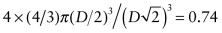 .
. - (c) As D = 0.2492 nm, the lattice constant =
 = 0.3524 nm.
 - (d) The mass of a nickel atom is 58.71/(6.022 × 1026) = 9.749 × 10⁻²⁶ kg. Hence the density = (4 × 9.749 × 10−26)/(0.3524 × 10−9)3 = 8911 kg/m3.
- E.4
- (a) Each corner atom is shared between 8 unit cells, and there is one atom at the cube centre. Hence the total number of atoms per unit cell is: 8 × (1/8) + 1 = 2 atoms.
Let the cubic unit cell have side length a. The length of the diagonal of the cube face is
 . Atoms touch on this diagonal, so this distance is also 2D, where D is the atomic diameter—hence
  . The atomic packing fraction is therefore:
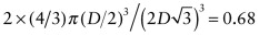
. This is lower than the value of 0.74 for FCC, which is close packed. BCC is not close packed.
- (b) As D = 0.2482 nm, the lattice constant =
 = 0.2866 nm.
 - (c) The mass of an iron atom is 55.85/(6.022 × 1026) = 9.274 × 10⁻²⁶ kg. Hence the density = (2 × 9.274 × 10−26)/(0.2866 × 10−9)3 = 7879 kg/m3.
- (a) Each corner atom is shared between 8 unit cells, and there is one atom at the cube centre. Hence the total number of atoms per unit cell is: 8 × (1/8) + 1 = 2 atoms.
- E.5 Figure GL1.18 shows how to calculate the octahedral hole size in the FCC structure. The face diagonals are close-packed directions, so the atom spacing along the diagonal is 1 unit. The cell edge thus has length
 = 1.414 units. That is also the separation of the centres of the atoms at opposite corners of the octahedral hole. The atoms occupy 1 unit of this, leaving a hole that will just contain a sphere of diameter 0.414 unit without distortion.
 - E.6 A tetrahedral hole of the HCP structure is sketched in Figure GL1.19.
- E.7 The indices of the planes are (a)
 , (b)
, (b)  , (c) (412).
 - E.8 The planes are parallel to the cube faces—the cleavage facets will meet at 90 degree.
- E.9 Figure GL1.20 shows the planes.
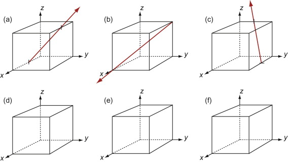
- E.10 The directions are (a) [011], (b)
 , (c)
, (c)  .
. - E.11 Figure GL1.21 shows the directions.
1 A more advanced and comprehensive ‘Teach Yourself Crystallography’ course can be down-loaded from the educational website Grantadesign.com/education/teachingresources.