
]>
Appendices
Appendix A: Hints for Simulations in Ansys HFSS
Ansys HFSS is industry standard software that is very popular for full-wave electromagnetic simulations. Simulations for lower frequency antennas below 10 GHz are straightforward, with no need for special consideration. But when designing mmWave antennas beyond 25 GHz, several aspects of simulations have to be examined. This section deals with hints for the simulation of Ka band antennas for 5G applications.
A.1Modelling
Care must be taken to use only lossy dielectrics and the actual conductor to be used. For example, copper of finite thickness is recommended rather than a perfect electric conductor (PEC) with no thickness. The dielectric loss tangent and conductor losses would lead to deterioration in the effective gain of the antenna [1,2,3]. The end-launch connector might be included in the modelling provided the computational resources for simulations support this. In most of the cases, a 50 Ω port impedance might suffice. The uncontrolled currents of the connector might influence the measurement results. The size of the radiation box must be fixed with respect to the lowest frequency of consideration for the sweep.
Figure A.1 illustrates the dialogue box for the solution setup for the Ka band antenna. The user must know a priori about the expected frequency of operation. If the structure is resonant, then a single frequency solution could be used. In the case of broadband structures, a corresponding radio button could be used. The solution frequency always has to be set as the highest frequency of sweep the user would be employing for simulations. For example, if the antenna is expected to operate from 25 to 40 GHz, the solution frequency must be set as 40 GHz. This strategy is to maintain the smallest size of the tetrahedron so that fine results could be achieved. The lower frequency setting in the solution frequency might result in a faulty shift in the resonant frequency. Also, a lower value is selected for solution frequency, so the effects of finer corners and corrugations might be totally missed by the simulation engine. The number of passes must be set at around 20–30, depending on the complexity of the geometry in simulation and the convergence criterion. The S-parameter error value could be set as 0.02; a finer value of this would give a better result but at the cost of greater time and computational resources.
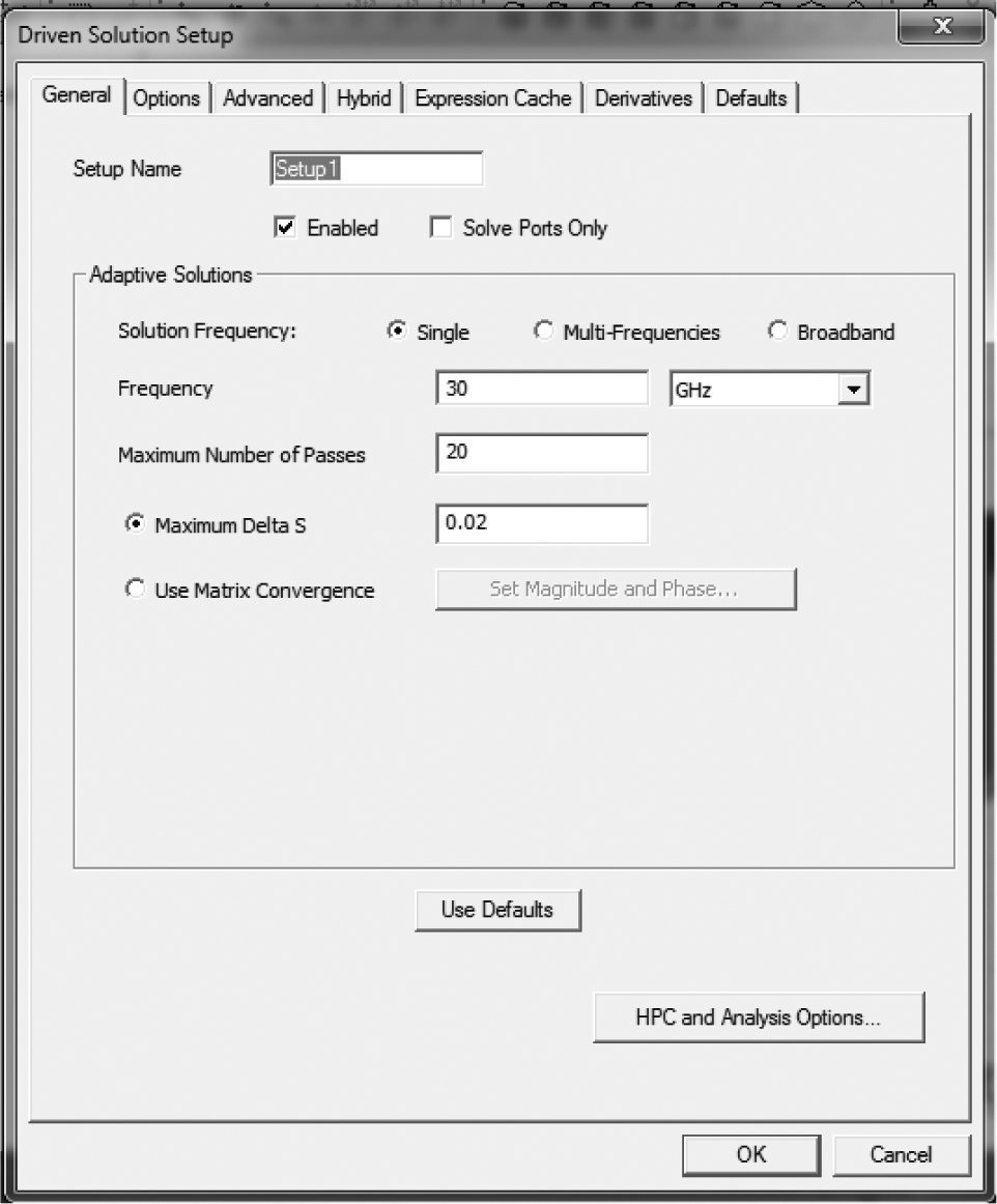
Figure A.1
Solution setup dialogue box for a 5G antenna in HFSS.
Figure A.2 illustrates the dialogue box of the validation check before simulation. The designer must verify that all the entities are validated. The software would also flag up issues in the warning and errors window. Post-simulation, the designer must verify that the convergence criterion has been met. A typical example is shown in Figure A.3; the target criterion was 0.02 and this was achieved, indicating minimal distortion in the simulated results.
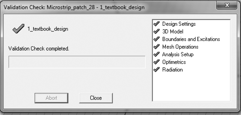
Figure A.2
Model validation dialogue box in Ansys HFSS.
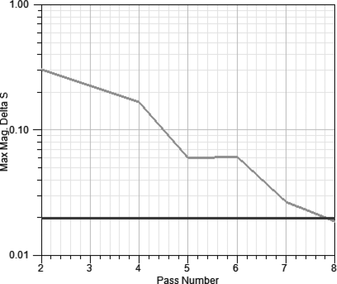
Figure A.3
Convergence curve from Ansys HFSS.
Analysis of the far field radiation patterns with respect to the antenna is an important aspect of simulations. Figure A.4 demonstrates the E-fields for a typical broadside radiator. The designer must anticipate the source of radiation by analysing the field lines of the entire antenna structure and the corresponding co-polarized and cross-polarized radiation patterns in the principal planes. It is critical to understand that all the field lines do not necessarily contribute to radiation. In this case, the patch antenna is an aperture radiator, wherein the radiation happens from the radiating edges, as shown by the solid lines near the inset of the patch. The field responsible for dominant co-polarized radiation is from Epat and the direction of wave propagation is along the Z-axis as indicated by k. Hence the pattern would lead to broadside radiation along the Z-axis. The principal cuts for this radiation are the XZ plane, which is scanning the E-plane, and the YZ plane, which is scanning the H-plane, as demonstrated in Figure A.5. The corresponding unit vectors for the principal cuts is also shown in the respective figures.
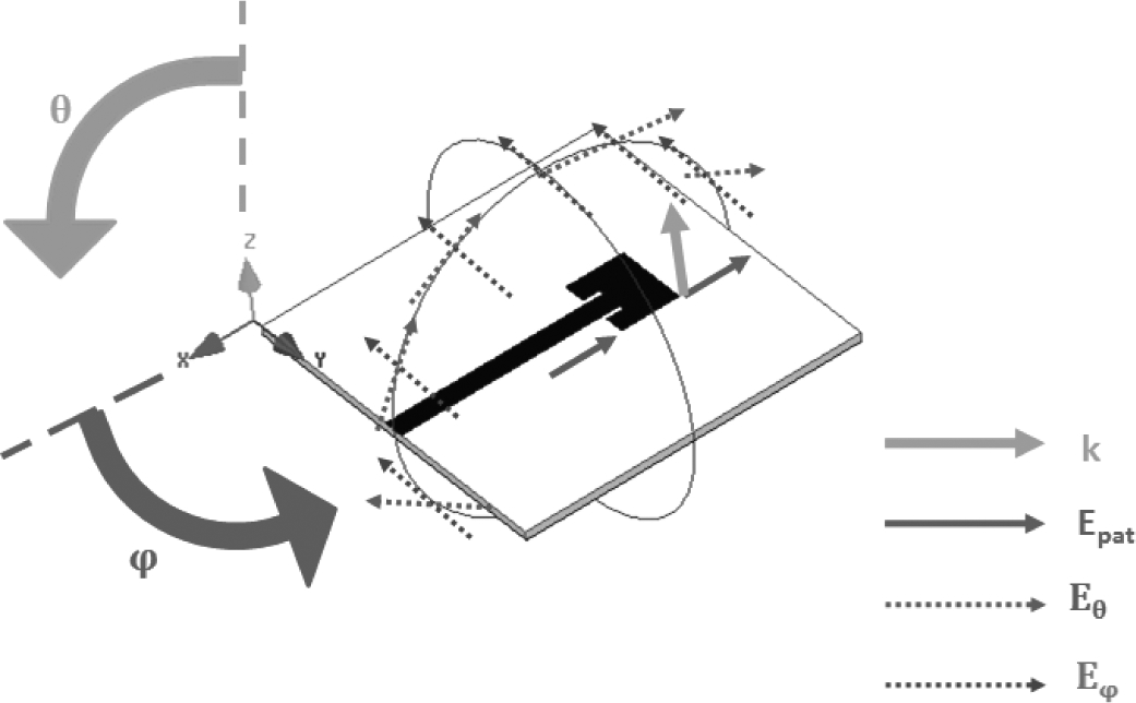
Figure A.4
Anatomy of E-fields for a broadside radiator for E-plane.
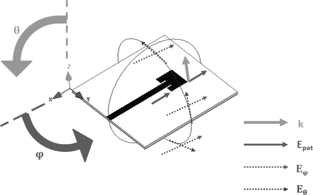
Figure A.5
Anatomy of E-fields for a broadside radiator for H-plane.
A tapered slot antenna is a typical end-fire radiator and the corresponding analysis of the radiation and its far-field is demonstrated in Figures A.6 and A.7.
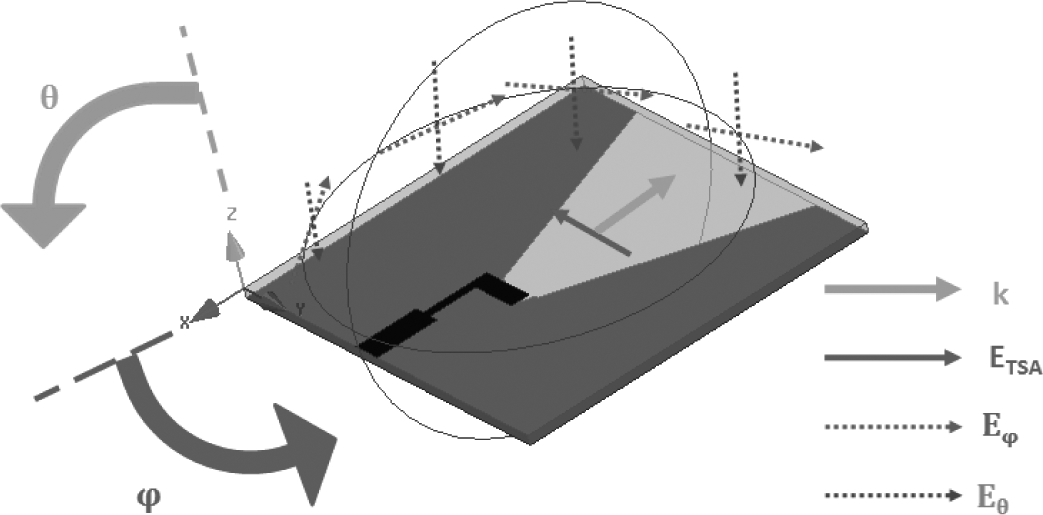
Figure A.6
Anatomy of E-fields for an end-fire radiator for E-plane.
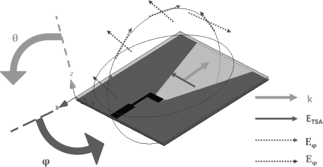
Figure A.7
Anatomy of E-fields for an end-fire radiator for H-plane.
Appendix B: Measurement Issues with End-Launch Connector
The connector assembly with the antenna or device under test is critical for measurements, especially in the Ka band [4–5]. Conventional commercial SMA connectors would operate up to 26.5 GHz. This does not mean that it would fail beyond the rated frequency. If the SMA connector could be soldered with a precision thin-tip soldering iron, then the possibility of it working would be higher. The trace of the SMA connector is close to 1 mm but most of the feed lines designed on electrically thin substrates have feed line widths much less than this, thus making assembly difficult. The mismatch between the traces might create additional distortion in the S-parameter’s measurement.
Hence end-launch connectors rated at 40 GHz are an ideal choice for the measurement of mmWave 5G antennas. The designer must allow ample clearance for the connector holes as per the official manual of the connector. Figure B.1 shows the exploded view of an end-launch connector. The primary entity has the trace pin and the upper ground mould. This trace pin must coincide with the feed line of the fabricated antenna. It is recommended that the trace pin must be soldered to the device under test. More often than not, soldering might not be necessary, as demonstrated in various chapters of this book. The grounding plates must be assembled precisely and fastened with an appropriate Allen key. An example of the assembled end-launch connector is shown in Figure B.2.
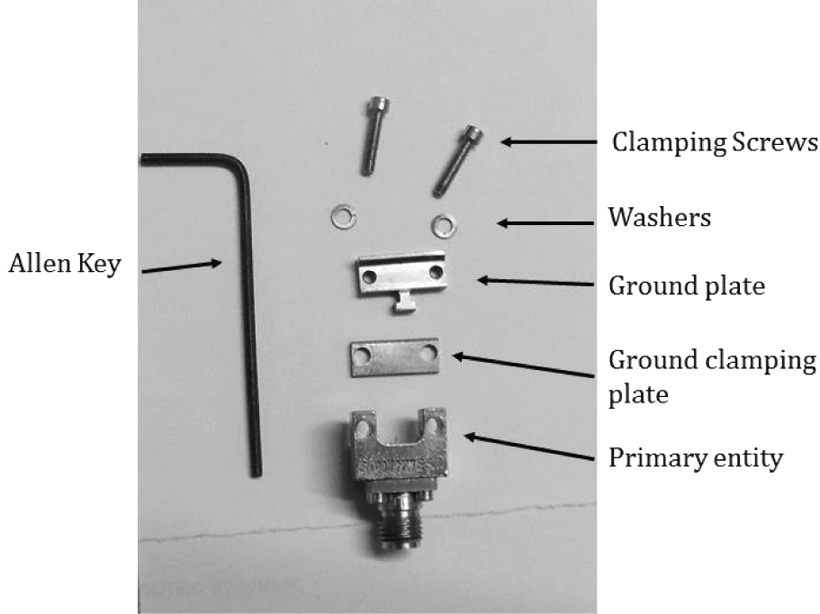
Figure B.1
Exploded view of part of an end-launch connector.
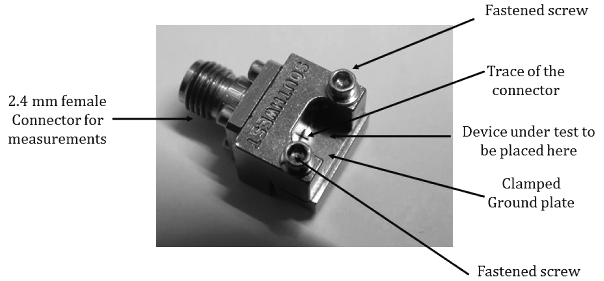
Figure B.2
Isometric view of an assembled end-launch connector.
Appendix C: Material Parameters’ Extraction Using S-parameters
The S-parameters simulation for a unit cell was explained in section 5.2.3. In this section, material parameters’ extraction using MATLAB is illustrated [6,7,8]. Initially, a Floquet port based simulation of the unit cell must be performed in HFSS. The data of real and imaginary components for the S-parameters of the unit cell simulation must be imported into the MATLAB workspace. Then the following code could be used for the extraction of material parameters.
S11=reS11+(i*imS11); %imported from the simulations of unit cell
S21=reS21+(i*imS21); %imported from the simulations of unit cell
d=5e-3;                % the primary distance between ports in HFSS
f=FreqGHz*1e9;        % convert to actual units, since HFSS exports in the GHz scale
lambda=(3e8)./f;      %calculate wavelength

% routine for calculation of mu and epsilon
% j is chosen to avoid the imaginary notation 'i'
% 51 discrete points were assumed in the simulation
for j=1:51
	K(j)=((S11(j)^2)-(S21(j)^2)+1)/(2*S11(j));
	Gamma(j)=K(j)-sqrt((K(j)^2)-1);
	T(j)=(S11(j)+S21(j)-Gamma(j))/(1-((S11(j)+S21(j))*Gamma(j)));
	Gumma(j)=(log(1/T(j)))/d;
	Gumma0(j)=i*((2*pi)/lambda(j));
	epsilon(j)=(Gumma(j)*(1-Gamma(j)))/(Gumma0(j)*(1+Gamma(j)));
	epsi(j)=conj(epsilon(j));
	mu(j)=(Gumma(j)*(1+Gamma(j)))/(Gumma0(j)*(1-Gamma(j)));
	mu_final(j)=conj(mu(j));
end

eps_Real=real(epsi);     % real value of epsilon
 figure(1);
 plot(FreqGHz,eps_Real);
 title('eps Real');
 figure(2);
eps_im=imag(epsi);       % imaginary value of epsilon
plot(FreqGHz,eps_im)
title ('eps imaginary');

 figure(3);
mu_real=real(mu_final); % real value of mu
plot(FreqGHz,mu_real);
title('mu_real');

figure(4);
mu_ima=imag(mu_final);
plot(FreqGHz,mu_ima);

figure(5);
plot(FreqGHz,eps_Real,'color','r'); hold on;
plot(FreqGHz,eps_im,'color','b');
title('permitivitty');

figure(6);
grid on;
plot(FreqGHz,mu_real,'color','r'); hold on;
plot(FreqGHz,mu_ima,'color','b');
title('permeability');
legend('real','imaginary');

figure(7);
grid on;
plot(FreqGHz,eps_Real,'color','r'); hold on;
plot(FreqGHz,eps_im,'color','b');
title('permitivitty');
legend('real','imaginary');
Appendix D: Useful MATLAB Codes
Aperture efficiency: to calculate the aperture efficiency of an antenna, it is important to initially understand the physical aperture of the antenna and then contemplate the actual gain [9,10]. Figure D.1 illustrates a broadside radiator integrated with a superstrate of dimensions L × W. The effective physical aperture of this topology could be identified as the physical area of the superstrate, hence Ap is the area of the superstrate, i.e., LW. From this entity the gain feasible from the physical aperture Gp could be calculated using Equation D.1, where λ is the wavelength in free space. The actual gain, Gact is the value from measurement or simulations. The ratio of actual gain to physical gain gives the aperture efficiency. It is imperative to divide the gain values in linear scale as against the logarithm scale, which leads to faulty high ratios.
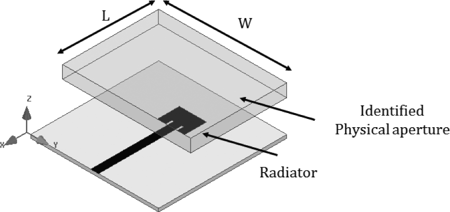
Figure D.1
Aperture efficiency for a broadside radiator.
Figure D.2 The scenario for a typical end-fire aperture ratio. The value of the physical aperture could be calculated using first principles or from the software.
Figure D.2
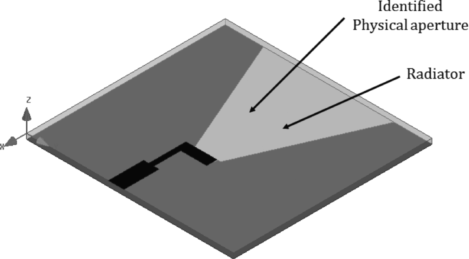
Aperture efficiency for an end-fire radiator.
The following MATLAB code is useful for extracting aperture efficiency.
f=FreqGHz*1e9;         % convert to actual units
lambda=(3e8)./f;       % calculate wavelength
Ap=180*1e-6; %in m^2   % Physical aperture either calculated or from HFSS
		       % j is chosen to avoid the imaginary nottaion 'i'
for j=1:21
   Gp(j)=(4*pi*Ap)/(lambda(j).^2);  % Gp calculation
   Ge(j)=Gain(j);                   % Gact (in linear scale) from HFSS
   Ae(j)=Ge(j)./Gp(j);              % Aperture efficiency as ratio
   Ae_percent(j)=Ae(j).*100;        % Aperture efficiency as percentage
end
The Envelope Correlation Coefficient (ECC) is an important metric when designing closely spaced antenna elements. The input reflection coefficient and the mutual coupling is extracted from HFSS. The following code could be used for ECC calculation.
S11=reS11+i*imS11;              % S11 imported from HFSS
S11_star=conj(S11);
S21=reS21+i*imS21;              % S21 imported from HFSS
S21_star=conj(S21);
modS11=magS11;
modS21=magS21;
S11_double=modS11.^2;
S21_double=modS21.^2;

for j = 1:51
   alpa(j)=(S11_star(j).*S21(j))+(S21_star(j).*S11(j));
   alpa2(j)=alpa(j).^2;
   deno(j)=(1-S11_double(j)-S21_double(j));
   ECC(j)=alpa2(j)./deno(j);
end
References
- 1.https://www.ansys.com/products/electronics/ansys-hfss.
- 2.https://www.ansys.com/-/media/ansys/corporate/ resourcelibrary/techbrief/ab-ansys-hfss-for-antenna -simulation.pdf?la=ja-jp&hash=5DDAE142D173937E4C 4946C0AB877EA1A856B401.
- 3.https://www.ansys.com/services/training-center/ electronics/ansys-hfss-getting-started.
- 4.https://mpd.southwestmicrowave.com/product- category/end-launch-connectors/.
- 5.https://mpd.southwestmicrowave.com/wp-content/ uploads/2018/07/Optimizing-Test-Boards-for-50-GHz-End -Launch-Connectors.pdf.
- 6.A. B. Numan and M. S. Sharawi, “Extraction of material parameters for metamaterials using a full-wave simulator [Education Column],” IEEE Antennas and Propagation Magazine, 55(5), 202–211, October 2013.
- 7.S. Arslanagic, T. V. Hansen, N. A. Mortensen, A. H. Gregersen, O. Sigmund, R. W. Ziolkowski, and O. Breinbjerg, “A review of the scattering-parameter extraction method with clarification of ambiguity issues in relation to metamaterial homogenization,” IEEE Antennas and Propagation Magazine, 55(2), 91–106, April 2013.
- 8.D. R. Smith, S. Schultz, P. Markos, and C. M. Soukoulis, “Determination of effective permittivity and permeability of metamaterials from reflection and transmission coefficients,” Physics Review B, 65(19), 195104, April 2002.
- 9.T. H. Jang, H. Y. Kim, I. S. Song, C. J. Lee, J. H. Lee, and C. S. Park, “A wideband aperture efficient 60-GHz series-fed E-shaped patch antenna array with copolarized parasitic patches,” IEEE Transactions on Antennas and Propagation, 64(12), 5518–5521, December 2016.
- 10.Y. He, N. Ding, L. Zhang, W. Zhang, and B. Du, “Short-length and high-aperture-efficiency horn antenna using low-loss bulk anisotropic metamaterial,” IEEE Antennas and Wireless Propagation Letters, 14, 1642–1645, 2015.