2

Problem Analysis in Mobile Communication System

2.1 Introduction to Wireless Channels

Apart from the transmitter and receiver circuit design issues, several other critical factors appear in the design of a mobile communication system, primarily due to the wireless channel and user mobility. A wireless channel is more complex than a traditional wired transmission channel, with lots of issues being involved in signal transmission through a wireless channel. Before discussing these issues in detail, first let us examine the basic working principles of a typical communication system. The information flow between two parties communicating is depicted in Figure 2.1. The information from the source is digitized, source coded (redundant bits are removed), passed through the protocol layers (where extra header bits are inserted), processed in the physical layer (channel coding, puncturing, interleaving, burst formation, etc.), modulated (converted into an analog signal), amplified, and sent via the channel. The signal propagates via the channel and finally reaches the receiver. The receiver receives the transmitted signal and reverses the operations to recover the source information. In this communication process, the channel plays a significant role, as its characteristics severely affect the signals that are propagated through it.

First let us try to understand how the signal transmission–reception process gradually becomes complex from a point-to-point – wire-line scenario to a multi-user – wireless – mobile scenario. In the case of a wired channel, it is typically copper wire that is used to connect the users with the local exchange. The problems associated with this are as follows. (1) Noise – this signal is unwanted to all receivers. It is mainly thermal noise that is the big issue here, which is generated due to temperature variations of the line and this noise gets added into the user's desired signal. The thermal noise distribution function is Gaussian in nature, so channel characteristics can be represented by a Gaussian channel. (2) Attenuation – this is because of the finite resistance of the copper wire. As discussed in Chapter 1, from Shannon's theory the capacity of the channel (C) can be written as C = B log (1 + S/N), where S is the signal strength and N is the noise at the receiver end. We design a receiver by defining the required link budget (the minimum S/N requirement) and set the transmitted power accordingly to meet this requirement. Defining this is easy and a one time job, as here the channel characteristics do not vary with respect to time.

The situation becomes little bit complex for the multi-user scenarios in a frequency division multiplexing system. In this scenario, the interference (the signal is wanted by at least one user and unwanted by the rest) from the other users comes into the picture. There are two types of interferences that occur in the frequency domain, and these are known as co-channel interference (CCI) and adjacent channel interference (ACI). In addition to this, in the time domain, there is inter-symbol interference (ISI), and this is generated, when the previous data signal overlaps with the next one, because of the delay spread and higher data rate, for example, a lesser symbol period.

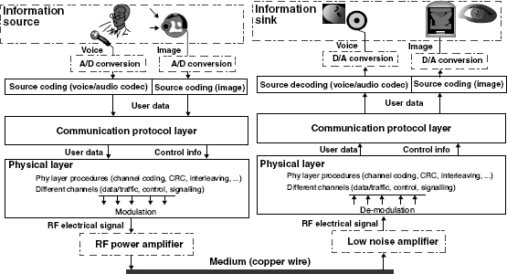
Figure 2.1 Information flow between two communicating parties

The situation becomes more complex in the case of a long range (r ~ 10 km for example, cellular system) wireless scenario. Here, apart from the path-loss and attenuation, there are several other phenomenon such as the multi-path effect (the same signal arrives at the receiver via different paths after multiple reflections and add up if they are in phase or cancel out if they are out of phase), shadow fading, interference, environment noise, burst noise, time dispersion or delay spread, and so on, seriously degrade the quality of the signal reception.

The situation become even worse in the mobile environment, as the the position of the receiver moves with respect to time, which causes the spread of the frequency bands due to the Doppler effect. There are two terms normally used to characterize the channel: (a) coherent time (T_c), which is the time interval over which the channel impulse response in essentially invariant, for example, over this period the channel does not change much; and (b) coherent bandwidth (B_c), which is the BW over which the channel transfer function remains virtually constant, for example, over this BW, all frequency bands will be equally affected by channel impairment.

As a result of all the phenomena discussed above, the received signal strength in a mobile wireless environment fluctuates from maximum to minimum. This is called signal fading and it makes the wireless channel extremely unpredictable. Shannon's capacity equation can be modified for a mobile wireless channel and can be represented, as C = B log (1 + |h|². S/N), where, |h|² is the channel gain and its value depends on the channel fading statistics. The major differences between a wireless and wire-line channel are summarized in Table 2.1.

The quality of a wireless link between the transmitter and a receiver depends on the radio propagation parameters, mobile environment and air channel's characteristics. Different problems arise due to various reasons at the transmitter, channel, and receiver locations:

• At Transmitter Variation of transmitter characteristics with respect to transmitted power, modulation, non-linearity of amplification, data rate, signal bandwidth, operating frequency and so on.

  Table 2.1 Differences between wire-line and wireless channels

  Wireless communication	Wire-line communication
  Air channel is used as the medium, which is a public channel	Generally, copper wire or fiber optic cables are used as medium and these are private channels (belonging to operator)
  Signal is transmitted as electromagnetic waves	Signal is transmitted as electrical signal
  The characteristic of air channel varies frequently with respect to time and frequency; the channel is unpredictable most of the time	The characteristic of wire channel does not vary much with respect to time (for example, over a long period of time, it is almost constant)
  Channel loss is more	Channel loss is less
  Generally receiver is mobile	Receiver is stationary
  Generally the channel is characterized by Rayleigh, Rician distribution	Generally channel is characterized by AWGN
  Security is a major threat	As the lines belong to specific operators, so although security is a major concern, it is less severe than wireless channel, where anyone can eavesdrop into the public air channel

• At Channel Variation of signal propagation in the unpredicted air channel due to attenuation, path loss, fading, multi-path, Doppler spread and so on.
• At Receiver Mobility of the receiver with respect to time and location, interference, noise, synchronization and so on.

All these factors are related to variability introduced by the mobile user because of signal reflection, diffraction, scattering, and a wide range of environmental variations that affect the signal propagation characteristics. These problems play a significant role in network, cell size, and receiver architecture design. In this chapter, we will first analyze various problems associated with communication over the wireless channel and then in Chapter 3, we will discuss various techniques or design solutions introduced to overcome these difficulties in wireless receivers across the generations of the wireless system.

2.2 Impact of Signal Propagation on Radio Channel

There are generally three basic phenomenon, reflection, diffraction, and scattering, which impact the signal propagation in a mobile wireless environment.

2.2.1 Reflection

Reflection occurs when a propagating electromagnetic wave impinges on a smooth surface of very large dimensions (>wavelength), as shown in Figure 2.2.

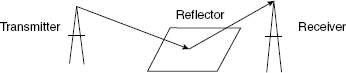
Figure 2.2 Reflection of a wave

2.2.2 Diffraction

Diffraction occurs when the radio path between the transmitter and the receiver is obstructed by a dense object with a sharp edge, causing deflection of the secondary waves in various directions away from the sharp edge, as shown in Figure 2.3. This forms secondary waves behind the obstructing body. Diffraction is a phenomenon that accounts for RF energy traveling from the transmitter to receiver without a line-of-sight path between the two. It is often termed shadowing because the diffracted field can reach the receiver even when shadowed by an impenetrable obstruction (Figure 2.3).

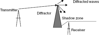
Figure 2.3 Diffraction of a wave

2.2.3 Scattering

Scattering occurs when a radio wave impinges on either a large rough surface or any surface whose dimensions are of the order of λ or less, causing the reflected energy to spread out (scatter) in all directions. This is shown in Figure 2.4. In an urban environment, typical signal obstructions that yield scattering are lampposts, street signs, and foliage (Figure 2.4).

Figure 2.4 Reflection of a wave

When the surface roughness increases a little, it creates two components: a specular reflection and a scattering component. The component of specular reflection is called the coherent component, while that of scattering is called diffuse or the incoherent component. However, when the surface roughness increases, only diffuse components will remain without any specular reflection component. Such surface scattering depends on the relationship between the wavelength of the electromagnetic radiation and the surface roughness, which is defined by the Rayleigh or Fraunhofer criteria. According to the Rayleigh criterion: if Δh < λ/8 cos θ, the surface is smooth. However, in the Fraunhofer criterion: if Δh < λ/32 cos θ, then the surface is smooth, where Δh is the standard deviation of surface roughness, λ is wavelength, and θ is the angle of incidence. Generally, the scattering coefficient, which is scattering per unit area, is a function of incident angle and scattering angle. Flat surface reflection coefficient (r_s) is multiplied by a scattering loss factor:

where Δh₀ = λ/(π cos θ), σ_h is the standard deviation of the surface height, I₀ is the modified Bessel function of first kind and zero order. The electric field, for minimum to maximum protuberance (h) > critical height (h_c) can be solved for a rough surfaces using the modified reflection co-efficient: Γ′ = Γ · r_s

2.3 Signal Attenuation and Path Loss

As discussed in Chapter 1, a transmitting antenna radiates a fraction of the given amount of power into free space. Considering the transmitter at the center of a radiating sphere (Omni directional radiation), the total power, which is found by integrating the radiated power over the surface of the sphere, must be constant regardless of the sphere's radius. After propagating a distance through the wireless channel from the transmitting antenna, some part of the signal impinges on the receiver antenna. For most antenna-based wireless systems, the signal also diminishes as the receiver moves away from the transmitter, because the concentration of radiated power changes with distance from the transmitting antenna.

Figure 2.5 Free space signal transmission

As shown in Figure 2.5, let us consider that the power P_t is fed to the transmitting antenna and it has a gain of G_t and also assume that the antenna is transmitting equally in all directions. Then the effective transmitter power (equivalent isotropic radiated power, EIRP) will be P_t* G_t. This power will be radiated over a sphere. At a distance R from the transmitter the sphere radius will be R and as the energy retention by the sphere is constant so the total energy over the sphere will always be same, for example, P_t·G_t. The energy density over the sphere will be P_tG_t/4 π R² and this indicates the received power at a distance R. Thus it is evident that when the receiver moves far away from the transmitter, R increases and received signal power P_r = P_tG_t/4 π R² decreases as a proportion of R². Also, if A is the effective area of the receiver antenna (where this transmitted wave will impinge), then the total received power at the receiving antenna will be:

Again, let us consider G_r is the gain of the received antenna. Thus:

If other losses are also present, then we can rewrite the above equation:

where L₀ is other losses expressed as a relative attenuation factor, and L_p is the free space path loss.

2.3.1 Empirical Model for Path Loss

Several empirical models exist for path loss computation, such as Okumura–Hata, COST 231 (Walfisch and Ikegami), and Awkward (graph) model. Amongst these, the Okumura–Hata model is the most widely used in radio frequency propagation for predicting the behavior of cellular transmissions in the outskirts of cities and other rural areas. The model calculates attenuation taking into account the percentage of buildings in the path, as well as any natural terrain features. This model incorporates the graphical information from the Okumura model and develops it further to suite the need better.

2.3.1.1 Okumura–Hata Model

Okumura analyzed path loss characteristics based on several experimental data collection around Tokyo, Japan. This model calculates the attenuation taking into account the parentage of buildings in the path, as well as the natural terrain features. Hata's equations are classified into three models as described below:

1. Typical Urban

   

   where a(h_m) is the correction factor for mobile antenna height and is given by

   For large cities:

   

   

   For small and medium cities:

   

2. Typical Suburban

   

3. Rural

   

where, f_c is the carrier frequency, d is the distance between the base station and the mobile handset (in km), h_b is the base station antenna height, and h_m is the mobile antenna height (in m).

2.3.1.2 COST 231 Model

The COST 231 model, also called the Hata model PCS extension, is a radio propagation model that extends the Hata and Okumura models to cover a more extensive range of frequencies. This model is applicable to open, suburban, and urban areas.

The model is formulated as:

where C = 0 dB for medium cities and suburban areas and 3 dB for metropolitan areas, L = median path loss (in dB), f = frequency of transmission (in MHz), h_B = base station antenna height (in m), d = link distance (in km), and C_H = mobile station antenna height correction factor.

2.4 Link Budget Analysis

Link budget is the budget of signal energy at the receiver on a given link accounting for all the risks in the link. A link budget relates TX power, RX power, path loss, RX noise and additional losses, and merges them into a single equation. A link budget tells us the maximum allowable path loss on each link, and helps to determine which link is the limiting factor. This maximum allowable path loss will help us to determine the maximum cell size. So, instead of solving for propagation loss in the prediction equations, we can take the maximum allowable loss from the link budget and calculate the cell radius R, from the propagation model. The link budget is simply a balance sheet of all the gains and losses on a transmission path, and usually includes a number of product gains/losses and “margins.” For a line of sight radio system, a link budget equation can be written as:

where P_RX = received power (dBm), P_TX = transmitter output power (dBm), G_TX = transmitter antenna gain (dBi), L_TX = transmitter losses (coax, connectors, …) (dB), L_FS = free space loss or path loss (dB), L_M = miscellaneous losses (fading margin, polarization mismatch, body loss, other losses, …) (dB), G_RX = receiver antenna gain (dBi), and L_RX = receiver losses (coax, connectors, …) (dB).

The receiver systems exhibit a threshold effect, when the signal to noise ratio (SNR) drops below a certain value (threshold value), the system either does not work at all, or operates with unacceptable quality. For acceptable performance, the necessary condition is: SNR (at receiver) ≥ threshold SNR, which indicates that P_r ≥ P_r0. P_r is limited by Equation 2.4 to provide satisfactory performance and P_r0 is receiver sensitivity.

As an example the parameters are analyzed here for a particular receiver:

1. Transmit Power – (>30–45 dBm for base stations and approximately 0–30 dBm for mobiles) this is simply the EIRP of the transmitter.
2. Antenna Gain – (>18 dBi for base stations) this is a measure of the antenna's ability to increase the signal.
3. Diversity Gain – (>3–5 dB) by utilizing various frequencies, time, or space, the system can extract signal information from other replicas and this translates into a gain.
4. Receiver Sensitivity – (>−102 to −110 dBm) the lowest signal that a receiver can receive and still be able to demodulate with acceptable quality.
5. Duplexer Loss – (>1 dB) the loss from using a duplexer unit, which duplexes the uplink and downlink.
6. Combiner Loss – (>3 dB) the loss from using a combiner unit, which combines multiple frequencies onto one antenna system.
7. Filter Loss – (>2–3 dB) the loss occurred due to the use of filters in the circuit.
8. Feeder Loss – (>3 dB) the loss from the cables connecting the base station with the antenna system.
9. Fade Margin – (>4–10 dB) this accounts for fading dips, especially for slow moving mobiles, because for fast moving mobiles they tend to move out of a dip faster than the channel changes. Some special curves (Jake's curves) are used to compute this parameter based on a certain reliability of coverage (percentage 75–95%).
10. Interference Margin – (>1 dB) this accounts for high interference from the other users.
11. Vehicle Penetration – (>6 dB) accounts for the attenuation of the signal by the chassis of a car.
12. Building Penetration – (>5–20 dB) accounts for the penetration of building material for indoor coverage. This depends on the type of building and the desired quality at the center of the interior.
13. User Body Loss – (>3 dB) accounts for the signal blockage created by a mobile user's head (sometimes called head loss).

Using tools such as Planet (MSI) or Wizard (Agilent) the coverage can be analyzed and we can also estimate co-channel and adjacent channel interference. The tools can be used for automatic frequency and code planning.

2.5 Multipath Effect

As many obstacles and reflectors (tall buildings, metallic objects, water surfaces, etc.) are present in a wireless propagation channel, so the transmitted signal is reflected by such reflectors and arrives at the receiver from various directions over multiple paths, as shown in Figure 2.6. Such a phenomenon is called a multipath. It is an unpredictable set of reflections and/or direct waves, each with its own degree of attenuation and delay. Multipath is usually characterized by two types of paths:

• Line-of-Sight (LOS) the straight line path of the wave from the transmitter (TX) directly to the receiver (RX).
• Non-Line-of-Sight (NLOS) the path of a wave arriving at the receiver after reflection from various reflectors.

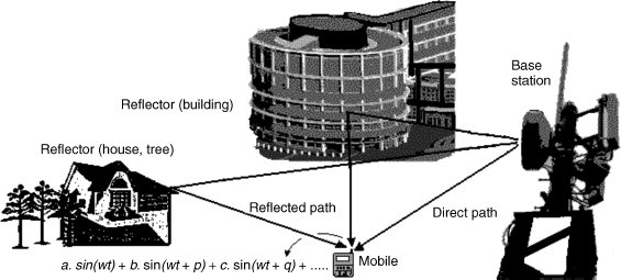
Figure 2.6 The multipath effect in a wireless channel

Multipath will cause fading (amplitude and phase fluctuations), and time delay in the received signals. When multipath signals are out of phase with the direct path signal, reduction of the signal strength at the receiver occurs; similarly when they are in phase, reinforcement of the signal strength occurs. This results in random signal level fluctuations, as the multipath reflections destructively (and constructively) superimpose on each other, which effectively cancels part of the signal energy for brief periods of time. The degree of cancellation, or fading, will depend on the delay spread of the reflected signals, as embodied by their relative phases, and their relative power. One such type of multipath fading is known as “Rayleigh fading” or “fast fading.”

2.5.1 Two Ray Ground Reflection Model

We will first consider two signals coming from the transmitter and one of them is reflected by a reflecting surface, whereas other one arrives directly at the receiver following the path d_D, as shown in Figure 2.7. The same principle can be extended to compute the resultant effect when considering multiple paths, because many such direct and reflected waves will arrive at the receiver.

Figure 2.7 The two ray reflection model in a wireless channel

Total received field at the receiver is:

where

where E_D = direct LOS component, E_R = reflected component, Δφ = phase difference, and Γ = complex reflection coefficient. The reflection introduces amplitude and phase fluctuation, for example, fading. The phase difference is:

As the mobile operating frequency (for example in GSM ~ 900 MHz) is very high. for example, the wavelength is smaller than the distance, so, we can assume:

where h₁ and h₂ are the height of the transmitter and receiver antenna. Thus the path difference ((d₁ + d₂) − d_D) = √((h_t + h_r)² + R²) − √((h_t − h_r) ² + R²). When R (h_t + h_r), then √((h_t + h_r)² +R²) − √((h_t − h_r)² + R²) = √[R²{((h_t + h_r)/R)² + 1} − √[R²{((h_t − h_r)/R)² + 1} = R·[√{((h_t + h_r)/R)² + 1} − √{((h_t + h_r)/R)² + 1}].

For small α (α 1), this indicates that Γ ≈ −1.

With this approximation, the total received field becomes:

It is important to observe that, as discussed earlier, in free space, as the distance R increases, the electric field decreases as 1/R and thus the power decreases as 1/R². However here, considering the multipath effect, the electric field reduces at a rate of 1/R². Hence the power reduces as 1/R⁴.

The path loss is

2.6 Delay Spread

To understand this, we should consider the effect of channel impulse response. In an ideal case, a Dirac pulse δ(t) is defined as δ(t) = 1, only at t = 0 and elsewhere δ(t) = 0. (However, in practice, the pulses are of finite width, as shown in Figure 2.8) If we assume a very short pulse of extremely high amplitude (delta pulse) is sent by the transmitting antenna at time t = 0 and considering a practical situation, this pulse will arrive at the receiving antenna via direct and numerous reflected paths with different delays τ_i and with different amplitudes (because of the different path distance and path loss). Thus, various parts of the pulse will arrive at the receiver at different instances in time based on the pulse width and the channel conditions. The impulse response of the radio channel is the sum of all the received pulses. Now, because of the mobility of the receiver (the receiver and some of the reflecting objects are also moving), the channel impulse response is a function of time and the delays (τ_i). The channel impulse response can be represented as:

The channel may vary with respect to time, which indicates that delta pulses sent at different instances (t_i) will cause different reactions in the radio channel. The delay spread can be calculated from the channel impulse response. As shown in Figure 2.9, for any practical channel the inevitable filtering effect will cause a spreading (or smearing out) of individual data symbols passing through a channel.

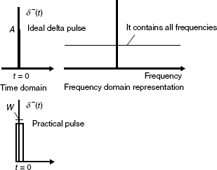
Figure 2.8 Nature of a delta pulse

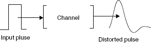
Figure 2.9 Channel delay spread

Two commonly used terms for delay spread calculations are the average and RMS delay spread and these are defined as below:

If power density is discrete as shown in Figure 2.10a, then the average and RMS delay spread for a multipath profile can be written as:

Figure 2.10 (a) Discrete power density, and (b) arrival of various multipath signals at different time scales

where

Thus delay spread is a type of distortion that is caused when identical signals (with different amplitudes) arrive at different times at the destination as shown in Figure 2.11 as. The signal usually arrives via multiple paths and with different angles of arrival. The time difference between the arrival moment of the first multipath component and the last one is called delay spread. This leads to time dispersion, resulting in inter symbol interference. This causes significant bit rate error, especially in the case of a TDMA based system.

Delay spread increases with frequency. The RMS delay spread is inversely proportional to the coherence bandwidth.

Figure 2.11 Delay spread

2.6.1 Coherent BW (Bc)

Coherence bandwidth is the bandwidth over which the channel transfer function remains virtually constant. This is a statistical measure of the range of frequencies over which the channel can be considered as “flat” (for example, a channel that passes all spectral components with approximately equal gain and linear phase). Equivalently, coherence bandwidth is the range of frequencies over which two frequency components have a strong potential for amplitude correlation. Formally the coherence bandwidth is the bandwidth for which the auto co-variance of the signal amplitudes at two extreme frequencies reduces from 1 to 0.5. For a Rayleigh fading WSSUS channel with an exponential delay profile, we can write, B_c = 1/(2 π σ_τ), where σ_τ is the RMS delay spread. This result follows on from the derivation of the correlation of the fading at two different frequencies. It is important to note that an exact relationship between coherence bandwidth and RMS delay spread does not exist. In general, spectral analysis techniques and simulation are required to determine the exact impact of a time varying multipath on a particular transmitted signal. Coherence BW characterizes the channel responses – frequency flat or frequency selective fading. The signal spectral components in the range of coherence bandwidth are affected by the channel in a similar manner.

2.7 Doppler Spread

If the mobile receiver moves away from or near to the transmitter with some velocity, then the approach velocity of EM wave changes based on its direction of movement (Figure 2.12). This leads to a change in frequency. This phenomenon is known as the Doppler effect. This means, in the case of a mobile receiver, due to the motion of the receiver and some reflecting objects in the medium, the receive frequency shifts as a result of the Doppler effect.

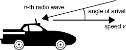
Figure 2.12 Mobile receiver and the Doppler effect

For single-path reception, this shift is calculated as follows:

where v = speed of the vehicle, c = speed of light, f_c = carrier frequency, α = angle between v and the line connecting the transmitter and receiver.

The Doppler shift = (v cos α)/λ, which is positive (resulting in an increase in frequency) when the radio waves arrive from ahead of the mobile unit, and is negative when the radio waves arrives from behind the mobile unit. The maximum Doppler shift = v/λ = f_m. Hence the above equation can be written as, f_d = f_m cos α. Doppler shift leads to (time varying) phase shifts of individual reflected waves. If it is for a single wave, then this minor shift does not bother radio system designers very much, as a receiver oscillator can easily compensate it. However, the fact is that many such waves arrive with different shifts. Thus, their relative phases change all the time, and so it affects the amplitude of the resulting received composite signal. Hence the Doppler effects determine the rate at which the amplitude of the resulting composite signal changes.

With multipath reception, the signals on the individual paths arrive at the receiving antenna with different Doppler shifts because of the different angles α_i, and the received spectrum is spread (spread in the frequency domain). The models behind Rayleigh or Rician fading assume that many waves arrive with their own random angle of arrival (thus with their own Doppler shift), which is uniformly distributed within [0, 2π], each independent of the other waves. This allows us to compute a probability density function of the frequency of the incoming waves. Moreover, we can obtain the Doppler spectrum of the received signal.

If the arrival angle α can be viewed as being uniformly distributed, then the Doppler frequency f_d = f_m cos α is cosine distributed. Received power in dα around α is proportional to dα/2π. Using

The Doppler power spectral density can be written as:

This implies that the Doppler shift causes frequency dispersion.

• Single frequency f_c broadened to a spectrum of (f_c − f_m, f_c + f_m).
• Signal with bandwidth 2B center at f_c broadened to a bandwidth of approximately 2B + 2 f_m.

Doppler spread B_D is defined as the “bandwidth” of the Doppler spectrum. It is a measure of spectral broadening caused by the time varying nature of the channel. The reciprocal of the Doppler spread is called the coherent time of the channel. Coherence time (T_c α 1/B_D), is used to characterize the time varying nature of the frequency dispersion of the channel in the time domain.

The effect of fading due to Doppler spread is determined by the speed of the mobile and the signal bandwidth. Let the baseband signal bandwidth be B_S and symbol period T_S, then

• “Slow fading” channel: T_S T_c or B_S B_D, signal bandwidth is much greater than Doppler spread, and the effects of Doppler spread are negligible.
• “Fast fading” channel: T_S > T_c or B_S < B_D, channel changes rapidly in one symbol period T_S.

Of course, other Doppler spectra are possible in addition to the pure Doppler shift; for example, spectra with a Gaussian distribution using one or several maxima. A Doppler spread can be calculated from the Doppler spectrum.

2.7.1 Coherence Time (T_c)

Coherence time is the time duration over which the channel impulse response is essentially invariant (Figure 2.13). If the symbol period of the baseband signal (reciprocal of the baseband signal bandwidth) is greater than the coherence time, then the signal will distort, as the channel will change during the transmission of a symbol of the signal.

We can say that this is the time interval within which the phase of the signal is (on average) predictable. Coherence time, T_c, is calculated by dividing the coherence length by the phase velocity of light in a medium; given approximately by T_c = λ²/(cΔλ), where λ is the central wavelength of the source, Δλ is the spectral width of the source, and c is the speed of light in a vacuum.

Coherence time characterizes the channel responses – slow or fast fading. It is affected by Doppler spread.

2.8 Fading

The fluctuation of signal strength (from maximum to minimum for example, deep) at the receiver due to the channel condition variation is known as fading. The effect of the channel on the various parameters of a signal is shown in Figure 2.14.

Figure 2.13 Coherence time (T_c)

Figure 2.14 Channel effect on the various parameters of a signal

Based on the signal fluctuation over distance scale, the fading can be classified into two categories:

2.8.1 Large-Scale Fading

Large-scale fading represents the average signal power attenuation or path loss. Free space attenuation, shadowing, causes large-scale fading. This is mostly dependent on prominent terrain contours (hills, forests, billboards, clumps of buildings, etc.) between the transmitter and receiver. The receiver is often represented as being “shadowed” by such prominences. This occurs, when the mobile moves through a distance of the order of the cell size. This is also known as “large-scale path loss,” “log-normal fading,” or “shadowing.” This is typically frequency independent.

2.8.2 Small-Scale Fading

Small-scale fading refers to fluctuations in the signal amplitude and phase that can be experienced as a result of small changes in distance between transmitter and receiver, due to constructive and destructive interference of multiple signal paths. This happens in a spatial scale of the order of the carrier wavelength. This is also known as “multipath fading,” “Rayleigh fading,” or simply as “fading.” Multipath propagation (delay spread), speed of the mobile (Doppler spread), speed of surrounding objects, and transmission bandwidth are the main factors that influence small-scale fading. This is typically frequency dependent.

A received signal, r(t), is generally described in terms of a transmitted signal s(t) convolved with the impulse response of the channel h_c(t). Neglecting the signal degradation due to noise, we can write r(t) = s(t) * h_c(t). In the case of mobile radios, r(t) can be partitioned in terms of two component random variables, as follows:

where m(t) is known as the large-scale fading component, and r₀(t) is the small-scale fading component (see Figure 2.15a). m(t) is sometimes referred to as the local mean or log-normal fading because the magnitude of m(t) is described by a log-normal pdf (or, equivalently, the magnitude measured in decibels has a Gaussian pdf). r₀(t) is sometimes referred to as multipath or Rayleigh fading.

Figure 2.15 (a) Large- and small-scale fading. (b) Classification of fading

As shown in Figure 2.15b, there are four main types of small-scale fading based on the following causes:

• Doppler Spread Causes
  1. - Fast Fading – High speed mobile environment that means high Doppler spread, coherence time < symbol period.
  2. - Slow Fading – Low speed that means low Doppler spread, coherence time > symbol period.
• Multipath Delay Spread Causes
  1. - Flat Fading – BW of signal < coherence BW, delay spread < symbol period.
  2. - Frequency Selective Fading – BW of signal > coherence BW, delay spread > symbol period.

We will discuss these below in more detail.

2.8.3 Flat Fading

If the mobile radio channel has a constant gain and linear phase response over a bandwidth that is greater than the bandwidth of the transmitted signal, which means B_s B_c or T_s σ_T, then under these conditions flat fading occurs (Figure 2.16). Flat-fading channels are also known as amplitude varying channels and are sometimes referred to as narrowband channels, as the BW of the applied signal is narrow when compared with the channel flat-fading BW.

Figure 2.16 Flat fading

Flat fading occurs when (a) signal BW coherence BW, and (b) T_s σ_T.

2.8.4 Frequency-Selective Fading

If the channel possesses a constant-gain and linear-phase response over a BW that is smaller than the BW of the transmitted signal, then the channel creates frequency-selective fading. Here, the bandwidth of the signal s(t) is wider than the channel impulse response (Figure 2.17).

Figure 2.17 Frequency selective fading

This occurs when (a) B_s > B_c and (b) T_s < σ_T. This causes distortion of the received baseband signal and inter-symbol interference (ISI).

2.8.5 Fast Fading

Fast fading occurs if the channel impulse response changes rapidly within the symbol duration. This means the coherence time of the channel is smaller than the symbol period of the transmitted signal. This causes frequency dispersion or time-selective fading due to Doppler spreading. The rate of change of the channel characteristics is larger than the Rate of change of the transmitted signal and the channel changes during a symbol period. In the frequency domain, the signal distortion due to fading increases with increasing Doppler spread relative to the bandwidth of the transmitted signal. Thus the condition for fast fading is:

The channel also changes because of receiver motion.

2.8.6 Slow Fading

Slow fading is the result of shadowing by buildings, mountains, hills, and other objects. In a slow-fading channel, the channel impulse response changes at a rate much slower than the transmitted baseband signal S(t). In the frequency domain, this implies that the Doppler spread of the channel is much less than the bandwidth of the baseband signals. Thus in this instance the channel characteristic changes slowly compared with the rate of the transmitted signal.

So, a signal undergoes slow fading if the following condition is satisfied”

where B_s = bandwidth of the signal, B_D = Doppler spread, T_s = symbol period, and T_c = coherence bandwidth.

The information is summarized in a Table 2.2, which will be very useful when designing any new wireless system.

Table 2.2 Different types of fading

Physical parameters:- v = velocity of mobile, c = velocity of light, Bs = transmitted signal bandwidth, Bc = coherence bandwidth, Tc = coherence time, Ds = Doppler shift, Td = delay spread
Physical parameters	Relations with other parameters
Doppler shift for a path (Ds)	Ds = fc·v/c
Coherence time (Tc)	Tc ~ 1/(4·Ds)
Coherence bandwidth (Wc)	Bc = 1/2·Td
Types of fading and defining characteristics
Fast fading	Tc delay requirement
Slow fading	Tc delay requirement
Flat fading	Bs Bc
Frequency selective fading	Bs Bc
Under spread channel	Td Tc

2.9 Signal Fading Statistics

For better receiver design, we want a statistical characterization to explain how quickly the channel changes, how much it varies, and so on. Such characterization requires a probabilistic model. Although the probabilistic models show poor performance for wireless channels, they are very useful for providing insight into wireless systems.

The fading distribution, describes how the received signal amplitude changes with time. It is a statistical characterization of the multipath fading. The received signal is a combination of multiple signals arriving from different directions, phases, and amplitudes. By received signal, we mean the baseband signal, namely the envelope of the received signal [r(t)]. Generally, three types of statistical distributions are used to describe fading characteristics of a mobile radio:

• Rayleigh distribution;
• Rician distribution;
• Log-normal distribution.

The rapid variations in signal power caused by a local multipath are represented by a Rayleigh distribution, whereas with an LOS propagation path, often the Rician distribution is used (Figure 2.18). Rician distributions describe the received signal envelope distribution for channels where one of the multipath components is a line-of-sight (LOS) component, that is, there is at least one LOS component present. A Rayleigh distribution describes the received signal envelope distribution for channels where all the components are non-LOS, that is, there is no LOS component and all are defused components. The long-term variations in the mean level are denoted by a log-normal distribution.

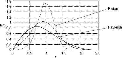
Figure 2.18 Rician density function and Rayleigh density function

2.9.1 Rician Distribution

When there is a dominant stationary (non-fading) LOS signal component present, then the small-scale fading envelope distribution is Rician. The Rician distribution degenerates to a Rayleigh distribution when the dominant component fades away.

In this case the probability distribution function (pdf) is given by:

where A is the peak amplitude of the dominant signal, and I₀ is the modified Bessel function of the first kind, and zero order, r²/2 = instantaneous power, and σ is the standard deviation of the local power. The Rician distribution is often described in terms of parameter K, which is known as the Rician factor and expressed as K = 10.log (A²/2 σ²) dB.

As A ≥ 0 and K ≥ α dB, because the dominant path decreases in amplitude, this generates a Rayleigh distribution.

2.9.2 Rayleigh Distribution

Typically this distribution is used to describe the statistical time varying nature of a received envelope of a flat-fading signal, or an envelope of individual multipath components.

Rayleigh distribution has the probability density function (pdf) given by:

where σ² is the average power of the received signal before envelope detection, and σ is the RMS value of the received voltage signal before envelope detection.

The Rayleigh-fading signal can be described in terms of the distribution function of its received normalized power, for example, the instantaneous received power divided by the mean received power = Φ = r²/2/σ².

As p(r) dr must be equal to p(Φ) dΦ, hence

This represents a simple exponential density function, which indicates that a flat-fading signal is exponentially fading in power. The average power is

Observations:

1. When A/σ = 0, the Rician distribution reduces to a Rayleigh distribution. As the dominant path decreases in amplitude, the Rician distribution degenerates to a Rayleigh distribution.
2. The Rician distribution is approximately Gaussian in the vicinity of r/σ, when A/σ is large.

2.9.3 Log-Normal Distribution

The log-normal distribution describes the random shadowing effects that occur over a large number of measurement locations which have the same transmitter and receiver separation, but have a different level of clutter on the propagation path. Typically, the signal s(t) follows the Rayleigh distribution but its mean square value or its local mean power is log-normal.

In many cases Nakagami-m distribution can be used in tractable analysis of fading channel performance. This is more general than Rayleigh and Rician.

Based on the channel fading type and speed of the mobile receiver, different types of channels are defined and used for channel simulation. For example, static channel (no fading, zero speed), RA100 (rural area, with a speed of 100 kmph), HT100 (hilly terrain, with a speed of 100 kmph), TU50 (typical urban, with a speed of 50 kmph).

2.10 Interference

In a multi-user scenario, different users communicate using the same medium. Under these conditions, every user's signal is considered as unwanted to the rest of the users (except to the intended receiver of that user's signal). We know that any unwanted signal is treated as noise. However, here in the true sense these signals are not noise, as this signal may be a wanted/desired signal for someone, for example, every signal has one intended receiver for which it was sent and the remainder may be unintended receivers of that signal. In a wireless system, one user's desired signal can interfere with another user's desired signal and corrupt it; this phenomenon of one user's desired signal interfering with another user's desired signal is known as interference. This means that one user is interfering with the others. Interferences arise due to various reasons, and although they corrupt the signals they are sometimes unavoidable.

2.10.1 Inter-Symbol Interference

The digital data are represented as a square pulse in the time domain. Figure 2.19 represents the digital signal of amplitude A and pulse width τ. Owing to the delay spread as described earlier, the transmitted symbol will spread in the time domain. For consecutive symbols this spreading causes part of the symbol energy to overlap with the neighboring symbols, which leads to inter-symbol interference (ISI).

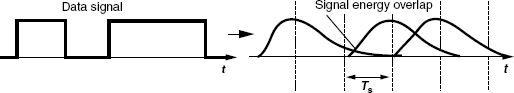
Figure 2.19 Inter-symbol interference

Ideally, a square wave in the time domain is a sync pulse in the frequency domain with infinite bandwidth. As all the practical communication systems are band-limited systems, there is always a certain amount of energy leak from the neighboring symbol and this amount is dependent on the bandwidth being used (refer to Chapter 4).

2.10.2 Co-Channel Interference

As the frequency is a very precious resource in wireless communication, in order to support many users, the same frequency is reused in some other distant cell. This reuse of frequency may cause an interference in another cell's mobile, where the same frequency is being used again. The co-channel interference occurs when two or more independent signals are transmitted simultaneously using the same frequency band.

In GSM, mobile radio operators have generally adopted a cellular network structure, allowing frequency reuse. The primary driving force behind this is the need to operate and support many users with the limited allocated spectrum. Cellular radio can be described as a honeycomb network set up over the required operating region, where frequencies and power levels are assigned in such a way that the same frequencies can be reused in cells, which are separated by some distance. This leads to co-channel interference problems. A co-channel signal that is at the same frequency band can easily bypass the RF filters and affects the energy level of the true signal. There will be more discussion on this in the Chapters 3 and 7.

2.10.3 Adjacent Channel Interference

Signals from nearby frequency channel (adjacent channel) leak into the desired channel and causes adjacent channel interference (Figure 2.20). This can be caused by bad RF filtering, modulation, and non-linearity within the electronic components. In such cases the transmitted signal is not really band limited, due to that the radiated power overlaps into the adjacent channels. To avoid this a guard band is generally inserted in between two consecutive frequency bands.

Figure 2.20 Adjacent channel interference

2.11 Noise

Any undesired signal is considered as a noise signal. The sources of noise may be internal or external (atmospheric noise, man made noise) to the system. In a receiver electrical circuit, this occurs as some electrons move in a random fashion, causing voltage/current fluctuations. In the case of a wireless channel, where the signal is not an electrical signal but rather it is an EM wave, hence the signal fluctuation, obstruction, environment RF interference, and superposition/mixing with other waves; all these disturbances (as discussed earlier) are also considered as noise. Here instead of signal to noise ratio (S/N), the signal/(interference + noise) ratio, and carrier/(interference + noise) ratio equations are used. As noise is random in nature it can only be predicted by statistical means, and usually shows a Gaussian probability density function as shown in Figure 2.21 is used for this.

Figure 2.21 Gaussian distribution function

The random motion of electrons causes votage and current fluctuation. As, the noise is random, so the mean value will be zero. Hence, we use the mean square value, which is a measure of the dissipated power. The effective noise power of a source is measured in root mean square (rms) values. Noise spectral density is defined as the noise content in a bandwidth of 1 Hz.

2.11.1 Noise in a Two-Port Circuit

To reduce noise added by a receiver system, the underlying causes of the noise must be evaluated. Broadband noise is generated and subsequently categorized by several mechanisms, including thermal noise and shot noise. Other causes include recombination of hole/electron pairs (G–R noise), division of emitter current between the base and the collector in transistors (partition noise), and noise associated with avalanche diodes. Noise analysis is based on the available power concepts.

Available Power This is defined as the power that a source would deliver to a conjugate matched load (maximum power transferred). Half the power is dissipated in the source and half the power is dissipated (transmitted) into the load under these conditions. As shown in Figure 2.22, a complex source is connected to a complex conjugate load. In this case the amount of power delivered can be easily computed. So if

this means that

then

Figure 2.22 Complex source connected to complex conjugate load

2.11.1.1 Power Measurement Units

Power gain in units of dB (decibel) = 10 log₁₀ (P_r/P_t), the log-ratio of the power levels of the two signals. This is named after Alexander Graham Bell and can also be expressed in terms of voltages, 20 log₁₀ (V_r/V_t), as P = (V²/R), where watts = 10 ^{dB mW/10} × 10⁻³.

2.11.2 Thermal Noise

When the temperature of a body increases, then the electrons inside it start flowing in a more zigzag fashion. This random motion of electrons in a conductor prevents the usual flow of current through the device and this type of unwanted signal generated as a result of temperature is known as thermal noise (Figure 2.23). This is proportional to the ambient temperature. Power is defined as the rate of energy removed or dissipated. The available power is the maximum rate at which energy is removed from a source and is expressed in joules/second (watt). The thermal noise power that is available is computed by taking the product of Boltzmann's constant, absolute ambient temperature, and the bandwidth (B) of the transmission path. Boltzmann's constant k is 1.3802 × 10⁻²³ J/K. With an increase in the ambient temperature, the electron vibration also increases, thus causing an increase in the available noise power. Absolute temperature (T) is expressed in degrees Kelvin. The thermal noise is expressed as P_W = kTB.

Figure 2.23 Thermal noise

2.11.3 White Noise

Noise where the power spectrum is constant with respect to frequency is called the white noise (Figure 2.24). Thermal noise can be modeled as white noise. An infinite-bandwidth white noise signal is purely a theoretical construction, as by having power at all frequencies, the total power of such a signal is infinite and therefore impossible to generate. In practice, however, a signal can be “white” with a flat spectrum over a defined frequency band (±10¹⁴ Hz).

Figure 2.24 Power spectrum of white noise

2.11.4 Flicker Noise

Flicker noise is associated with crystal surface defects in semiconductors and is also found in vacuum tubes. The noise power is proportional to the bias current and unlike thermal and shot noise, flicker noise decreases with frequency, for example, when the frequency is less, the flicker noise is more (Figure 2.25). An exact mathematical model does not exist for flicker noise, because it is so device-specific. However, the inverse proportionality with frequency is almost exactly 1/f for low frequencies, whereas for frequencies above a few kilohertz, the noise power is weak but essentially flat. Flicker noise is essentially random, but because its frequency spectrum is not flat, it is not a white noise. It is often referred to as pink noise because most of the power is concentrated at the lower end of the frequency spectrum. Because of this, metal film resistors are a better choice for low-frequency, low-noise applications, as carbon resistors are prone to flicker noise.

Figure 2.25 Flicker noise defined by corner frequency

2.11.5 Phase Noise

Phase noise describes the short-term random frequency fluctuations of an oscillator. Phase noise is the frequency domain representation of rapid, short-term, random fluctuations in the phase of a wave (in RF engineer's terms), caused by time domain instabilities (“jitter” in a digital engineer's terms). An ideal oscillator would generate pure sine waves but all real oscillators have phase modulated noise components in them. The phase noise components spread the power of a signal to adjacent frequencies, resulting in sidebands. Typically this is specified in terms of dBc/Hz (amplitude referenced to a 1-Hz bandwidth relative to the carrier) at a given offset frequency from the carrier frequency.

Phase noise is injected into the mixer LO (local oscillator) port by the oscillator signal as shown in Figure 2.26. If perfect sinusoidal signals are input to the RF port, the LO signal and its phase noise mixes with the input RF signals and produces IF (intermediate frequency) signals containing phase noise. If a small desired signal f_d and a large undesired signal f_u are input to the RF port, the phase noise on the larger conversion signal may mask the smaller desired signal and this would hinder reception of the desired signal. Thus, low phase noise is crucial for oscillators in receiver systems. During the detection of digitally modulated signals, the phase noise also adds to the RMS phase error.

2.11.6 Burst Noise

Burst noise or popcorn noise is another low frequency noise that seems to be associated with heavy metal ion contamination. Measurements show a sudden shift in the bias current level that lasts for a short duration before suddenly returning to the initial state. Such a randomly occurring discrete level burst would have a popping sound if amplified in an audio system. Like flicker noise, popcorn noise is very device specific, so a mathematical model is not very useful. However, this noise increases with bias current level and is inversely proportional to the square of the frequency 1/f².

Figure 2.26 Frequency conversion limitation due to phase noise

2.11.7 Shot Noise

This noise is generated by current flowing across a P–N junction and is a function of the bias current and electron charge. The impulse of charge q depicted as a single shot event in the time domain can be Fourier transformed into frequency domain as a wideband noise.

where I₀ is the dc current and e = electron charge = 1.6 × 10⁻¹⁹ coulomb.

The power produced by shot noise is directly proportional to the bias current. Like thermal noise, shot noise is purely random and its power spectrum is flat with respect to frequency (Figure 2.27). Measurements confirm that the mean-square value of shot noise is given by

Figure 2.27 Shot noise

where I_n = rms average noise current in amperes, q = 1.6 × 10⁻¹⁹ coulombs (C), the average/electron, I_dc = dc bias current in the device in amperes, B = bandwidth in which measurement t is made, in Hz.

2.11.8 Avalanche Noise

Avalanche noise occurs in zener diodes, because in reverse biased P–N junctions the breakdown happens after a certain voltage. This noise is considerably larger than shot noise, so if zeners have to be used as part of a bias circuit then they need to be RF decoupled.

2.11.9 Noise Figure (NF)

This is the ratio of the signal to noise at the input to the signal to noise at the output of a device. This indicates how much extra noise has been added to the signal by the device. The noise figure is represented as:

Noise figure (NF) is a measure of the degradation of the signal to noise ratio (SNR), caused by the components in the device circuit. Noise figure is always greater than 1, and the lower the noise figure the better the device. When T is the room temperature represented by T_o (290 K), and noise temperature is T_e, then the factor (1 + T_e/T_o) is called the noise figure of an amplifier.

The noise figure is the decibel equivalent of noise factor: F = 10^NF/10, where NF = 10 log (F). If several devices are cascaded, the total noise factor can be found using the Friis formula:

where F_n is the noise factor for the nth device and G_n is the power gain (numerical, not in dB) of the nth device. This indicates that the NF of the first block should be as minimal as possible to keep the noise under control. This is why one low noise amplifier is placed in the receiver circuit at the first stage to boost the signal strength without increasing the overall noise level.

Further Reading

Goldsmith, A. (2005) Wireless Communications, Cambridge University Press, Cambridge.

Rappaport, T.S. (1996) Wireless Communications: Principles and Practice, Prentice Hall, Englewood, NJ, ISBN 9780133755367.

Tse, D. and Viswanath, P. (2005) Fundamentals of Wireless Communication, Cambridge University Press, Cambridge.