1

Introduction to Mobile Handsets

1.1 Introduction to Telecommunication

The word telecommunication was adapted from the French word télécommunication, where the Greek prefix tele- (τηλε-) means- “far off,” and the Latin word communicare means “to share.” Hence, the term telecommunication signifies communication over a long distance. In ancient times, people used smoke signals, drum beats or semaphore for telecommunication purposes. Today, it is mainly electrical signals that are used for this purpose. Optical signals produced by laser sources are recent additions to this field. Owing to the evolution of major technological advances, today telecommunication is widespread through devices such as the television, radio, telephone, mobile phone and so on. Telecommunication networks carry information signals from one user to another user, who are separated geographically and this entity may be a computer, human being, teleprinter, data terminal, facsimiles machine and so on. The basic purpose of telecommunication is to transfer information from one user to another distant user via a medium. God has given us two beautiful organs: one is an eye to visualize things and other is an ear to listen. So, to the end users, in general information transfer is either by voice or as a real world image. Thus, we need to exchange information through voices, images and also computer data or digital information.

1.1.1 Basic Elements of Telecommunication

The basic elements of a telecommunication system are shown in the Figure 1.1. In telephonic conversation, the party who initiates the call is known as the calling subscriber and the party who is called is known as the called subscriber. They are also known as source and destination, respectively. The user information, such as sound, an image and so on, is first converted into an electrical signal using a transducer, such as a microphone (which converts sound waves into an electrical signal), a video camera (which converts an image into an electrical signal) and so on, which is then transmitted to the distant user via a medium using a transmitter. The distant user receives the signal through the use of a receiver and this is then fed to an appropriate transducer to convert the electrical signal back into the respective information (for example, a speaker is used as a transducer on the receiver side to convert the electrical signal into a sound wave or the LCD display is used to convert the electrical signal into an image).

Before getting into an in-depth discussion, we will first familiarize ourselves with some of the most commonly used terms and mathematical tools for mobile telecommunication system design and analysis. We will learn about some of these as we progress through the various chapters.

Figure 1.1 Basic elements of telecommunication

1.1.1.1 Signal

The amplitude of a time varying event is described as a signal. Using Fourier's theory a signal can be decomposed into a combination of pure tones, called sine or cosine waves, at different frequencies. Different sine waves that compose a signal can be plotted as a function of frequency to produce a graph called a frequency spectrum of a signal. The notion of a sinusoid with exponentially varying amplitude can be generalized by using a complex exponential. Based on the nature of the repetition of the signal amplitude with respect to time, the signal can be classified as periodic (repeats with every period) and aperiodic (not a periodic waveform). Also, signals can be either continuous or discrete in nature with respect to time.

Analog Signal

Analog signals are continuous with time as shown in Figure 1.2. For example, a voice signal is an analog signal. The intensity of the voice causes electric current variations. At the receiving end, the signal is reproduced in the same proportions.

Figure 1.2 Analog and digital signal

As shown in the Figure 1.3, the signal can be represented in complex cartesian or polar format. Here, T is period of a periodic signal (T = 1/frequency) and A is the maximum amplitude. ω_o is the angular frequency (=2πf ) and Φ is the phase at any given instant of time (here at t = 0).

Signals having the same frequency follow the same path (repeat on every period T), but different points on the wave are differentiated by phase (leading or lagging). From the figure it is obvious that one period (T ) is 360° of a phase (a complete rotation). Harmonics (2f, 3f, …) are waves having frequencies that are integer multiples of the fundamental frequency. These are harmonically related exponential functions.

Figure 1.3 Signal representation in polar and cartesian format

Digital Signal

Digital signals are non-continuous with time, for example, discrete. They consist of pulses or digits with discrete levels or values. The value of each pulse width and amplitude level is constant for two distinct types, “1” and “0”, of digital values. Digital signals have two amplitude levels, called nodes and the value of which is specified as one of two possibilities, such as 1 or 0, HIGH or LOW, TRUE or FALSE and so on. In reality, the values are anywhere within specific ranges and we define the values within a given range. A system which uses a digital signal for processing the information is known as a digital system. A digital system has certain advantages over an analog system, as mentioned below.

Advantages – (1) Digital systems are less affected by any noise signal compared with analog signals. Unless the noise exceeds a certain threshold, the information contained in digital signals will remain intact. (2) In an analog system, aging and wear and tear will degrade the information that is stored, but in a digital system, as long as the wear and tear is below a certain level, the information can be recovered perfectly. Thus, it is easier to store and retrieve the data without degradation in a digital system. (3) It provides an easier interface to a computer or other digital devices. Apart from this ease of multiplexing, ease of signaling has made it more popular.

Disadvantages – From their origins, voice and video signals are analog in nature. Hence, we need to convert these analog signals into the digital domain for processing, and after processing again we need to convert them back into the original form to reproduce. This leads to processing overheads and information loss due to conversions.

Digital Signaling Formats

The digital signals are represented in many formats, such as non-return to zero, return to zero and so on, as shown in Figure 1.4. In telecommunication, a non-return-to-zero (NRZ) line code is a binary code in which “1s” are represented by one significant condition and “0s” are represented by the other significant condition, with no other neutral or rest condition. Return-to-zero (RZ) describes a line code used in telecommunications signals in which the signal drops (returns) to zero between each pulse. The NRZ pulses have more energy than an RZ code, but they do not have a rest state, which means a synchronization signal must also be sent alongside the code.

Unipolar Non-Return-to-Zero (NRZ) – Here, symbol “1” is represented by transmitting a pulse of constant amplitude for the entire duration of the bit interval, and symbol “0” is represented by no pulse. This allows for long series without change, which makes synchronization difficult. Unipolar also contains a strong dc component, which causes several problems in the receiver circuits, such as dc offset.

Figure 1.4 Digital signal representations

Bipolar Non-Return-to-Zero – Here, pulses of equal positive and negative amplitudes represent symbols “1” and “0.” (for example, ± A volts). This is relatively easy to generate. Because of the positive and negative levels, the average voltage will tend towards zero. So, this helps to reduce the dc component, but causes difficulties for synchronization.

Unipolar Return-to-Zero – Symbol “1” is represented by a positive pulse of amplitude A and half symbol width and symbol “0” is represented by transmitting no pulse.

Bipolar Return-to-Zero – Positive and negative pulses of equal amplitude are used alternatively for symbol “1,” with each pulse having a half-symbol width; no pulse is used for symbol “0.” The “zero” between each bit is a neutral or rest condition. One advantage of this is that the power spectrum of the transmitted signal has no dc components.

Manchester Coding – In the Manchester coding technique, symbol “1” is represented by a positive pulse followed by a negative pulse, with each pulse being of equal amplitude and a duration of half a pulse. The polarities of these pulses are reversed for symbol “0.” An advantage of this coding is that it is easy to recover the original data clock and relatively less dc components are present. However, the problem is it requires more bandwidth. For a given data signaling rate, the NRZ code requires only half the bandwidth required by the Manchester code.

1.1.1.2 Analog to Digital Conversion

To convert an analog signal into a digital signal an electronic circuit is used, which is known as an analog-to-digital converter (ADC). Similarly, to convert a digital signal into an analog signal, a digital to analog converter (DAC) is used. The concept is depicted in Figure 1.5. Most of the ADCs are linear ADC types, where the range of the input values map to each output value following a linear relationship. Here, the levels are equally spaced throughout the range, whereas in the case of non-linear ADC, all the levels are not equally spaced. So, in this case, the space where the information is most important is sampled with a lesser gap and space, and where information is important, it is sampled at a higher rate. Normally, a compander (compressors and expanders) is used for this purpose. An 8-bit A-law or the μ-law logarithmic ADC covers the wide dynamic range. ADCs are of different types; below a few of the commonly used ADCs are discussed.

Figure 1.5 Analog to digital and digital to analog conversion

1. Direct conversion ADC (flash ADC) – As shown in Figure 1.6, this consists of a bank of comparators; each one outputs their decoded voltage range, which is then fed to a logic circuit. This generates a code for each voltage range. This type of ADC is very fast, but usually it has only 8 bits of resolution (with 256 comparators). For higher resolution, it requires a large number of comparators, this leads to larger die size and a high input capacitance, which makes it expensive and prone to produce glitches at the output. This is often used for wideband communications, video or other fast signals conversion.

   

   Figure 1.6 Flash analog to digital converter

2. Sigma–delta ADC – This works using two principles: over sampling and noise shaping. The main advantage of this filter is its notch response. It offers low cost, high resolution, and high integration. This is why this is very popular in the present day's mobile receivers. This is discussed in detail in Chapter 10.

1.1.1.3 Sampling

The process of converting a continuous analog signal into a numeric sequence or discrete signal (or digital signal) is known as sampling. A sample refers to a value or set of values, at a point in time and/or space. The discrete sample instance may be spaced either at regular or irregular intervals.

Sampling Interval – A continuous signal varies with time (or space) and the sampling is done simply by measuring the value of the continuous signal at every T units of time (or space), and T is called the sampling interval. Thus the sampling frequency (fs) = 1/T.

Sampling Rate and Nyquist Theorem – For a single frequency periodic signal, if we sample at least two points over the signal period, then it will be possible to reproduce a signal using these two points. Hence the minimum sampling rate is f_s = 2/T = 2f. A continuous function, defined over a finite interval can be represented by a Fourier series with an infinite number of terms as given below:

However, for some functions all the Fourier coefficients become zero for all frequencies greater than some frequency value – f_H. Now, let us assume that the signal f (x) is a band-limited signal with a one-sided baseband bandwidth f_H, which means that if f (x) = 0 for all | f | > f_H, then the condition for exact reconstruction of the signal from the samples at a uniform sampling rate f_s is, f_s > 2f_H. Here, 2f_H is called the Nyquist rate. This is a property of the sampling system (see Figure 1.7). The samples of f (x) are denoted by: x[n] = x(nT ), n N (integers). The Nyquist sampling theorem leads to a procedure for reconstructing the original signal x(t) from its samples x[n] and states the conditions that are sufficient for faithful reconstruction. Nyquist, a communication engineer in Bell Telephone Laboratory in 1930, first discovered this principle. In this principle, it is stated as “Exact reconstruction of a continuous-time baseband signal from its samples is possible, if the signal is band-limited and the sampling frequency is greater than twice the signal bandwidth.”

On the other side, the signal is being recovered by a sample and hold circuit that produces a staircase approximation to the sampled waveform, which is then passed through the reconstructive filter. The power level of the signal coming out of the reconstructive filter is nearly same as the level of the original sampled input signal. This is shown in the Figure 1.8.

Aliasing – If the sampling condition is not satisfied, then the original signal cannot be recovered without distortion and the frequencies will overlap. So, frequencies above half the sampling rate will be reconstructed as, and appear as, frequencies below half the sampling rate. As it is a duplicate of the input spectrum “folded” back on top of the desired spectrum that causes the distortion, this is why this type of sampling impairment is known as “foldover distortion” and the resulting distortion is also called aliasing. For a sinusoidal component of exactly half the sampling frequency, the component will in general alias to another sinusoid of the same frequency, but with a different phase and amplitude. The “eye pattern” is defined as the synchronized superposition of all possible realizations of the signal of interest viewed within a particular signaling interval. It is called such because the pattern resembles the human eye for binary waves. The width of the eye opening defines the time interval over which the received signal can be sampled without error from inter-symbol interference.

Figure 1.7 Sampling frequency

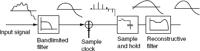
Figure 1.8 Sampling and reconstruction of signal

As shown in Figure 1.9, if we sample x(t) too slowly, then it will overlap between the repeated spectra resulting in aliasing for example, we cannot recover the original signal, so aliasing has to be avoided. To prevent or reduce aliasing, two things need to be taken into consideration. (1) Increase the sampling rate more than or equal to twice the maximum signal frequency (whatever the maximum signal frequency present in that band is). (2) Introduce an anti-aliasing filter or make the anti-aliasing filter more stringent.

Although we want the signal to be band-limited, in practice, however, the signal is not band-limited, so the reconstruction formula cannot be precisely implemented. The reconstruction process that involves scaled and delayed sinc functions can be described as an ideal process. However, it cannot be realized in practice, as it implies that each sample contributes to the reconstructed signal at almost all time points, which requires summing an infinite number of terms. So, some type of approximation of the sinc functions (finite in length) has to be used. The error that corresponds to the sinc-function approximation is referred to as the interpolation error. In practice digital-to-analog converters produce a sequence of scaled and delayed rectangular pulses, instead of scaled, delayed sinc functions or ideal impulses. This practical piecewise-constant output can be modeled as a zero-order hold filter driven by the sequence of scaled and delayed Dirac impulses referred to the mathematical basis. Sometimes a shaping filter is used after the DAC with zero-order hold to give a better overall approximation.

Figure 1.9 Signal distortion (energy overlap) due to low sampling rate

When the analog signal is feed to the ADC based on the maximum and minimum value of the analog signal amplitude, the range of the analog signal is defined and the resolution of the converter indicates the number of discrete values that it can produce over the range of analog values. The values are usually stored in binary form, hence it is expressed in the number of bits. The available range is first divided into several spaced levels, and then each level is encoded into n number of bits. For example, an ADC with a resolution of 8 bits can encode an analog input to one in 256 different levels, as 2⁸ = 256. The values can represent the ranges from 0 to 255 (that is, unsigned integer) or −128–127 (that is, signed integer), depending on the application.

1.1.1.4 Accuracy and Quantization

The process of quantization is depicted in Figure 1.10. The signal is limited to a range from VH (15) to VL (0), and this range is divided into M (=16) equal steps. The step size is given by, S = (VH − VL )/M.

The quantized signal Vq takes on any one of the quantized level values. A signal V is quantized to its nearest quantized level. It is obvious that the quantized signal is an approximation to the original analog signal and an error is introduced in the signal due to this approximation. The instantaneous error e = (V − Vq ) is randomly distributed within the range (S/2) and is called the quantization error or noise. The average quantization noise output power is given by the variance σ² = S²/12.

The toll quality speech is band limited to 300–3400 Hz (speech signal normally contains signals with a frequency range in between 300 and 3400 Hz). To digitize this waveform the minimum sampling frequency required is 2 × 3400 Hz = 6.8 KHz in order to avoid aliasing effects. The filter used for band limiting the input speech waveform may not be particularly ideal with a sharp cut off, thus a guard band is provided and it is sampled at a rate of 8 KHz.

Dithering – The performance of ADC can be improved by using dither, where a very small amount of random noise (white noise) is added to the input signal before the analog to digital conversion. The amplitude of this is set to be about half of the least significant bit. Its effect is to cause the state of the LSB to oscillate randomly between 0 and 1 in the presence of very low levels of input, instead of sticking at a fixed value. So, effectively the quantization error is diffused across a series of noise values. The result is an accurate representation of the signal over time.

Figure 1.10 Quantization process

Sample Rate Converter – Sampling rate changes come in two types: decreasing the sampling rate is known as decimation and when the sampling rate is being increased, the process is known as interpolation. In the case of multimode mobile devices, the sample rate requirement is different for different modes. In some instances, where one clock rate is a simple integer multiple of another clock rate, resampling can be accomplished using interpolating and decimating FIR filters. However, in most situations the interpolation and decimation factors are so high that this approach is impractical. Farrow resamplers offer an efficient way to resample a data stream at a different sample rate. The underlying principle is that the phase difference between the current input and wanted output is determined on a sample by sample basis. This phase difference is then used to combine the phases of a polyphase filter in such a way that a sample for the wanted output phase is generated. Compared with single stage, a multi-stage sampling rate conversion system offers less computation and more flexibility in filter design.

1.1.1.5 Fourier Transforms

At present, almost every real world signal is converted into electrical signals by means of transducers, such as antennas in electromagnetics, and microphones in communication engineering. The analysis of real world signals is a fundamental problem. The traditional way of observing and analyzing signals is to view them in the time domain. More than a century ago, Baron Jean Baptiste Fourier showed that any waveform that exists in the real world can be represented (and generated) by adding up the sine waves. Since then, we have been able to build (or break down) our real world time signal in terms of these sine waves. It has been shown that the combination of sine waves is unique and any real world signal can be represented by a combination of sine waves, also there may be some dc values (constant term) present in this. The Fourier transform (FT) has been widely used in circuit analysis and synthesis, from antenna theory to radiowave propagation modeling, from filter design to signal processing, image reconstruction, stochastic modeling to non-destructive measurements.

The Fourier transform allows us to relate events in the time domain to events in the frequency domain. We know that various types of signals exist, such as periodic, aperiodic, continuous and discrete. There are several versions of the Fourier transform, and are applied based on the nature of the signal. Generally, Fourier transform is used for converting a continuous aperiodic signal from the time to frequency domain and a Fourier series is used for transforming a periodic signal. For aperiodic–discrete signal (digital), discrete time Fourier transform is used and for periodic–discrete signals that repeat themselves in a periodic fashion from negative to positive infinity, the discrete Fourier series (most often called the discrete Fourier transform) is used.

The transformation from the time domain to the frequency domain is based on the Fourier transform. This is defined as:

Similarly, the conversion from frequency domain to time domain is called inverse Fourier transform, which is defined as:

Here s(t), S(ω), and f are the time signal, the frequency signal, and the frequency, respectively, and j = √−1, angular frequency ω = 2πf. The FT is valid for real or complex signals, and in general, it is a complex function of ω (or f ). Some commonly used functions and their FT are listed in Table 1.1

Table 1.1 Some commonly used functions and their Fourier transforms

Time domain	Frequency domain
Rectangular window	Sinc function
Sinc function	Rectangular window
Constant function	Dirac Delta function
Dirac Delta function	Constant function
Dirac comb (Dirac train)	Dirac comb (Dirac train)
Cosine function	Two, real, even Delta function
Sine function	Two, imaginary, odd Delta function
Exp function −{jexp(jωt)}	One, positive, real Delta function
Gaussian function	Gaussian function

1.1.1.6 System

A system is a process for which cause (input) and effect (output) relations exist and can be characterized by an input–output (I/O) relationship. A linear system is a system that possesses the superposition property, for example, y(t) = 2x(t), and an example of non-linear system is y(t) = x²(t) + 2x(t).

Time-invariant system: a time shift in the input signal causes an identical time shift in the output signal.

Memory-less (instantaneous) system: if present output value depends only on the present input value.

Otherwise, the system is called memory (dynamic) system.

Causal system (physically realizable system): if the output at any time t₀ depends only on the values of input for t ≤ t₀. For example, if x₁(t) = x₂(t) for t ≤ t₀, then y₁(t) = y₂(t) for t ≤ t₀.

Stable system: a signal x(t) is said to be bounded if |x (t)| < B < for any t. A system is stable, if the output remains bounded for any bounded inputs, this is called bounded-input bounded-output (BIBO) stable system.

Practical system: a non-linear, time-varying, distributed and non-invertible.

1.1.1.7 Statistical Methods

When a signal is transmitted through the channel, two types of imperfections can cause the received signal to be different from the transmitted signal. Of these, one is deterministic in nature, such as linear and non-linear distortion, inter symbol interference and so on, but the other one is nondeterministic, such as noise addition, fading and so on, and we model them as random processes.

The totality of the possible outcomes of a random experiment is called the sample space of the experiment and it is denoted by S. An event is simply a collection of certain sample points that is subset of the sample space. We define probability P as a set function assigning non-negative values to all events E, such that the following conditions are satisfied:

1. 0≤P(E)≤1 for all events
2. P(S ) = 1
3. For disjoint events E1, E2, E3, …, we have

A random variable is a mapping from the sample space to the set of real numbers. A random variable X is a function that associates a unique numerical value X(λ_i) with every outcome λ_i of an event that produces random results. The value of a random variable will vary from event to event, and, based on the nature of the event, it will be either continuous or discrete. Two important functions of a random variable are cumulative distribution function (CDF) and probability density function (PDF).

The CDF, F(X ) of a random variable X is given by

where P[X(λ) ≤ x] is the probability that the value X(λ) taken by the random variable X is less than or equal to the quantity x.

The PDF, f (x) of a random variable X is the derivative of F(X) and thus is given by

From the above equations, we can write

The average value or mean (m) of a random variable X, also called the expectation of X, is denoted by E(X). For a discrete random variable (X_d), where n is the total number of possible outcomes of values x₁, x₂, …, x_n, and where the probabilities of the outcomes are P(x₁), P(x₂), …, P(x_n), it can be shown that

For a continuous random variable X_c, with PDF f_c(x), it can be represented as

The mean square value can be represented as

A useful number to help in evaluating a continuous random variable is one that gives a measure of how widely its values are spread around its mean. Such a number is the root mean square value of (X − m) and is called the standard deviation σ of X.

The square of the standard deviation, σ², is called the variance of X and is given by

The Gaussian (or normal PDF) is very important in wireless transmission. The Gaussian probability density function f (x) is given by

when m = 0 and σ = 1 the normalized Gaussian probability density function is achieved.

1.1.1.8 Basic Information Theory

Information theory was developed to find the fundamental limits on data compression and reliable data communication. It is based on probability theory and statistics. A key measure of information in the theory is known as information entropy, which is usually expressed by the average number of bits needed for storage or communication. The entropy is a measure of the average information content per source symbol. The entropy, H, of a discrete random variable X is a measure of the amount of uncertainty associated with the value of X. If X is the set of all messages x that X could be, and p(x) is the probability of X given x, and then the entropy of X is defined as

In the above equation, I(x) is the self-information, which is the entropy contribution of an individual message. The special case of information entropy for a random variable with two outcomes is the binary entropy function:

We assume that the source is memory-less, so the successive symbols emitted by the source are statistically independent. The entropy of such a source is

From the above equation, we can observe

1. When p₀ = 0, the entropy = 0, when p₀ = 1, the entropy = 0.
2. The entropy H_b(p) attains its maximum value H_max = 1 bit, when p₁ = p₀ = 1/2 for example, symbol 0 and 1 are equally probable. This is shown in Figure 1.11.

Figure 1.11 Entropy function H(p)

A binary symmetric channel (BSC) with crossover probability p is a binary input, binary output channel that flips the input bit with probability p. The BSC has a capacity of 1 − H_b(p) bits per channel use, where H_b is the binary entropy function as shown in the Figure 1.12.

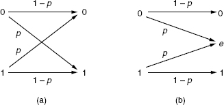
Figure 1.12 (a) A binary symmetric channel with crossover probability p is a binary input. (b) A binary erasure channel (BEC) with erasure probability p is a binary input

A binary erasure channel (BEC) with erasure probability p is a binary input, ternary output channel. The possible channel outputs are 0, 1, and a third symbol “e” called an erasure. The erasure represents complete loss of information about an input bit. The capacity of the BEC is 1 − p bits per channel use.

Let p(y|x) be the conditional probability distribution function of Y for a given X. Consider the communications process over a discrete channel, for example, X represents the space of messages transmitted, and Y the space of messages received during a unit time over our channel. The appropriate measure to maximize the rate of information is the mutual information, and this maximum mutual information is called the channel capacity and is represented by:

1.1.1.9 Power and Energy of a Signal

The energy (and power) of a signal represent the energy (or power) delivered by the signal when it is interpreted as voltage or current source feeding a 1 ohm resistor. The energy content of a signal x(t) is defined as the total work done and is represented as:

The power content of a signal is defined as work done over time and is represented as:

Conventionally, power is defined as energy divided by time. A signal with finite energy is called an energy-type signal and a signal with positive and finite power is a power-type signal. A signal is energy type if E(x) < ∞ and is power type if 0 < P < ∞.

1.1.1.10 Bandwidth (BW)

The signal occupies a range of frequencies. This range of frequencies is called the bandwidth of the signal. In general, the bandwidth is expressed in terms of the difference between the highest and the lowest frequency components in the signal. A baseband signal or low pass signal bandwidth is a specification of only the highest frequency limit of a signal. A non-baseband bandwidth is the difference between the highest and lowest frequencies.

As the frequency of a signal is measured in Hz (Hertz), so, the bandwidth is also expressed in Hz. Also, we can say that the bandwidth of a signal is the frequency interval, where the main part of the power of the signal is located. The bandwidth is defined as the range of frequencies where the Fourier transform of the signal has a power above a certain amplitude threshold, commonly half the maximum value (half power ~−3 dB, as 10 log₁₀(P/P_half) = 10 log₁₀ (1/2) = −3. Power is halved (P/2) at the 3 dB points for example, P = P/2 = (V₀/√2)(I₀/√2), where V₀ and I₀ are the peak amplitude of voltage and current, respectively; refer to Figure 1.13.

However, in digital communication the meaning of “bandwidth” has been clouded by its metaphorical use. Technicians sometimes use it as slang for baud, which is the rate at which symbols may be transmitted through the system. It is also used more colloquially to describe channel capacity, the rate at which bits may be transmitted through the system.

Bit Rate – This is the rate at which information bits (1 or 0) are transmitted. Normally digital system require greater BW than analog systems.

Baud – The baud (or signaling) rate defines the number of symbols transmitted per second. One symbol consists of one or several bits together, based on the modulation technique used. Generally, each symbol represents n bits, and has M signal states, where M = 2ⁿ. This is called M-ary signaling.

1.1.1.11 Channel Capacity

The maximum rate of communication via a channel without error is known as the capacity of the channel. In a channel where noise is present, there is an absolute maximum limit for the bit rate of transmission. This limit arises when the number of different signal levels is increased, as in such a case the difference between two adjacent sampled signal levels becomes comparable to the noise level. Claude Shannon extended Nyquist's work to a noisy channel.

Figure 1.13 Bandwidth of a signal

Applying the classic sphere scenario, we can obtain an estimate of the maximum number of code words that can be packed in for a given power constant P, within a sphere of radius √(NP). The noise sphere has a volume of √(Nσ²). Thus, as shown in the Figure 1.14, the maximum number of code words that can be packed in with non-overlapping noise spheres is the ratio of the volume of the sphere of radius √{(Nσ²) + NP)}, to the volume of the noise sphere: [√{(Nσ²) + NP)}]^N/[√(Nσ²)]^N, where, N is the signal space dimension and σ² is the variance of the real Gaussian random variable with mean μ. This equation implies that the maximum number of bits per symbol that can be reliably communicated is

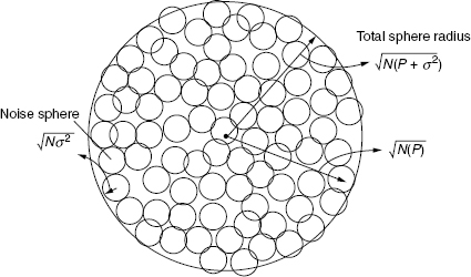
Figure 1.14 Number of noise spheres that can be packed into N dimensional signal space

This is indeed the capacity of the AWGN (additive white Gaussian noise) channel. In later chapters, we will see that for complex channels, the noise in I and Q components is independent. So it can be thought of as two independent uses of a real AWGN channel. The power constraint and noise per real symbol are represented as P_av/2B and N₀/2, respectively. Hence the capacity of the channel will be

This is the capacity in bits per complex dimension or degrees of freedom. As there are B complex samples per second, the capacity of the continuous time AWGN channel is

Now, the signal to noise ratio (SNR) = (P_av/N₀·B) – which is the SNR per degree of freedom. So, the above equation reduces to

This equation measures the maximum achievable spectral efficiency through the AWGN channel as a function of the SNR.

1.2 Introduction to Wireless Telecommunication Systems

The medium for telecommunication can be copper wire, optical fiber lines, twin wire, co-axial cable, air or free space (vacuum). To exchange information over these mediums, basically the energy is transferred from one place to the other. We know that there are two ways by which energy can be transferred from one place to another: (1) through the bulk motion of matter or (2) without the bulk motion of matter, which means via waves. With waves the energy/disturbance progresses in the form of alternate crests and troughs. Again, the waves are of two types: (1) mechanical waves and (2) electromagnetic waves. A mechanical wave can be produced and propagated only in material mediums that posses elasticity and inertia. These waves are also known as elastic waves; a sound wave is an example of an elastic wave. An electromagnetic wave does not require any such material medium for its propagation, it can travel via free space; light is an example of an electromagnetic wave. This is why we see the light from the sun, but do not hear any sound of bombardments from the sun.

In a conventional wire-line telephone system, the wire acts as the medium through which the information is carried. However, with a wireless system, as the name WIRELESS indicates, there is no wire, so removes the requirement for a wire between the two users. This means that the information has to be carried via air or free space. Thus the air or free space medium will be used for transmitting and receiving the information. But, what will help to carry the information through this free space or air? The answer was given in the previous paragraph – electromagnetic waves. As electromagnetic waves can travel through free space and air, we can use electromagnetic waves to send–receive information. Thus we conclude that for wireless communication, air or free space will be used as the channel/medium and electromagnetic waves will be used as the carrier. Then next problem to arise is how to generate this electromagnetic (EM) wave?

1.2.1 Generation of Electromagnetic Carrier Waves for Wireless Communication

In 1864 James Clark Maxwell theoretically predicted the existence of EM waves from an accelerated charge. According to Maxwell, an accelerated charge creates a magnetic field in its neighborhood, which in turn creates an electric field in this same area. A moving magnetic field produces an electric field and vice versa. These two fields vary with time, so they act as sources of each other. Thus, an oscillating charge having non-zero acceleration will emit an EM wave and the frequency of the wave will be same as the oscillation of the charge.

Twenty years later, in the period 1879–1886, after a series of experiments, Heinrich Hertz come to the conclusion that an oscillatory electrical charge q = q_o sin ωt radiates EM waves and these waves carry energy. Hertz was also able to produce EM waves of frequency 3 × 10¹⁰ Hertz. The experimental setup is shown in the Figure 1.15. To detect EM waves, he also used a loop S, which is slightly separated as shown in the figure. This is the basis for the theory of antenna.

Figure 1.15 Hertz experiment, generation of EM wave

In 1895–1897, Jagdish Bose also succeeded in generating EM waves of very short wavelength (~25 mm). Marconi, in Italy in 1896, discovered that if one of the spark gap terminals is connected to an antenna whilst the other terminal is earthed, then under these conditions the EM waves can travel up to several kilometers. This experiment launched a new era in the field of wireless communication.

So, now we know that an antenna is the device that will help to transmit and receive the EM waves though the air or free space medium. Next, we will see how the antenna actually does this.

1.2.2 Concept of the Antenna

An antenna is a transducer that converts electrical energy into an EM wave or vice versa. Thus, an antenna acts as a bridge between the air/free-space medium (where the carrier is the EM wave) and the communication radio device (where the energy is carried in the form of low frequency electrical signals). From network theory, we know that if the terminated impedance is matched with a port, then only the maximum power will be transmitted to the load, otherwise a significant fraction of it will be reflected back to the source port. Basically, the antenna is connected to a communication device port, so the impedance should be matched to transfer maximum power; similarly on the other side, the antenna is also connected to the air/free-space, so the impedance should be matched on that side to transfer maximum power.

Physically, an antenna is a metallic conductor, it may be a small wire, a slot in a conductor or piece of metal, or some other type of device.

1.2.2.1 Action of an Antenna

When an ac signal is applied to the input of an antenna, the current and voltage waveform established in the antenna is as shown in the Figure 1.16. This is shown for a length of a wire of λ/2.

Figure 1.16 Charge, current and voltage distribution

If the length changes then the distribution of charge on the wire will also change and the current–voltage waveform will also change. In Figure 1.17, various waveforms for different antenna lengths are shown. Wherever the voltage is a maximum, then the current is a minimum as they are 90° out of phase.

Figure 1.17 Voltage and current distribution across the antenna conductor for different lengths

It is evident that the minimum length of an antenna required to transmit or receive a wave effectively will be at least λ/4. This is because the property of a periodic wave resides mainly in any section of length “λ/4” and then it repeats over an interval of λ/4. This means that by knowing only λ/4 of a wave, we can reconstruct the wave. Basically, the distance between the maxima and minima of a signal waveform is λ/4, so all the characteristics of the wave will remain there.

How Does the EM Wave Carry Energy Over a Long Distance? – As shown in Figure 1.18, when an RF (radio frequency) signal is applied to the antenna, at one instant of time (when the signal is becoming positive- (a)), conductor A (the dipole) of the antenna will be positive due to a lack of electrons, and at that instant B will be negatively charged due to the accumulation of electrons. As the end points of A and B is an open circuit, so charge will accumulate over there. From the Maxwell equations, we know that electrical flux lines always start from the + ve point and end at the −ve point, and form a closed loop. A current flowing through a conductor produces a magnetic field and voltage produces an electric field. So, lines of electric and magnetic fields will be established across the antenna conductors as shown in Figure 1.18a.

Figure 1.18 Creation of flux lines with the RF signal variation

In the next instance of time (b), when the applied input RF signal decreases to zero, at this time there is no energy to sustain the closed flux loops of the magnetic and electric field lines, which were created in the previous instance of time. So, these will detach from the antenna and remain self sustained.

In the next instance of time (c), when A becomes negative and B positive, the electric and magnetic flux lines will be created again, but this time the direction will be reversed, as the + ve and −ve points are interchanged. Now, when the RF signal goes to zero, these flux lines again becomes free and self sustained.

The flux lines that were created in the first instance when A was positive and B was negative will have the opposite direction to the flux lines that were created when A is −ve and B is + ve. Thus, these flux lines will repel each other, and will move way from the antenna as shown in Figure 1.19.

Figure 1.19 Signal reception by the antenna

This phenomenon is repeated again and again according to the variation with time of the input radio frequency (RF) signal (for example, according to its frequency) and a series of detached electric and magnetic fields move onwards from the transmitting antenna.

In a 3D space (free space) these flux lines will actually be spherical in shape. If the radius of the sphere is r, and the power of the RF signal (V*I) during the time when these flux lines were generated is P_t, then the power P_t is spread over the surface of a sphere whose radius is r, so the power density will be P_t/4πr². Taking this energy, the flux lines will move away from the transmitting antenna. Now, as they move away from the antenna, the size of the sphereincreases, r increases but the same power (P_t) is contained within it. Thus the power density P_t/4π·r² decreases as it travels far from the transmitting antenna (for example, increase in r), and the problem of transmission of electrical energy via air/free-space is solved.

How is Energy Received on the Other Side? – Again, the antenna helps to solve this problem too. It transforms the received EM wave into an electrical signal. When the transmitted wave arrives at the receiving end, it tries to penetrate via another the metallic antenna. We know that the EM wave consists of an electric field and a magnetic field and that these are perpendicular to each other, and also that they are perpendicular to the direction of propagation. Thus when the EM wave touches the metallic antenna (from Maxwell's third equation) the magnetic field (H) will generate a surface current on the metallic antenna, which will try to penetrate via the metal (as it is a good conductor). However, it will die down after traveling a thickness of the skin depth, and, the EM wave will generate an electrical current in the metal body of the antenna. Similarly (from Maxwell's fourth equation), the electric field will generate an electric voltage in the antenna, as shown in Figure 1.19.

This phenomenon can be experienced by placing a radio inside a closed metallic chamber and finding that it does not play, as the EM wave can not penetrate via the thick metallic wall. However, it can penetrate through a concrete wall. For the same reason, a mobile telephone call disconnects inside an enclosed metallic lift due to the degradation of the signal strength.

Thus we have converted the transmitted energy (which was transmitted using the carrier of the EM waves) back into the electrical signal through the help of another antenna. So the antenna helped in transmitting and receiving the information through the air. As the user wants to send and receive the information, ideally the user should have both transmitting and receiving antennas. However, in general, in a mobile device, the same antenna is used for transmission as well as receiving purposes (refer to Chapter 4).

Thus we now know how to transmit and receive the information via the air (for example, via a wireless medium) using antenna. However, the problem at this stage is whether the baseband signal is transmitted directly, as its frequency is low (~KHz), and so it can not be sent directly via the air due to the following problems:

1. A larger antenna length (~λ/4) is required.
2. Much less BW is available at the lower frequency region.

The solution to this is to up-convert the baseband signal to a high frequency RF signal at the transmitter and then similarly down-convert at the receiver for example, which requires RF conversion techniques. How is the baseband signal up-converted/down-converted? The solution for up-conversion is the use of analog or digital modulation and mixing techniques (on a transmitter block) and the solution for down-conversion is the use of demodulation mixing techniques (on a receiver block). These will be discussed in more detail in Chapter 4. Next we will establish what else, apart from the antenna, is required inside the transmitter and receiver to transmit or receive the information.

1.2.3 Basic Building Blocks of a Wireless Transmitter and Receiver

We know that a digital system is more immune to noise, and that in addition to this there are many such advantages of digital systems over the old analog systems. So, from the second generation onwards wireless systems have been designed with digital technology. However, there is a problem, in that voice and video signals are inherently analog in nature. So how can these signals be interfaced with a digital system? These signals have to be brought into the digital domain for processing using an analog-to-digital converter (ADC) and then again reverted back into an analog signal using a digital-to-analog converter (DAC) and then sent via an antenna. A typical transmitter block diagram of a wireless system is shown in the Figure 1.20.

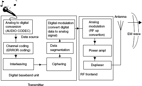
Figure 1.20 Transmitter system block diagram

As shown in the Figure 1.20, on the transmitter side, when the user speaks in front of a microphone, it generates an electrical signal. This signal is sampled and converted into digital data and then fed to the source codec, for example, a speech codec unit (this is discussed in more details in Chapter 8), which removes the redundant data and generates the information bits. These data are then fed into the channel coder unit. When the signal travels via the medium, during this time it can be affected by signal noise, so we need some type of protection against this. The channel coder unit inserts some extra redundant data bits using an algorithm, which helps the receiver to detect and correct the received data (this is discussed in more detail in Chapter 3). Next, it is fed to an interleaving block. When data pass through the channel, this time there may be some type of burst noise in the channel, which can actually corrupt the entire data during this burst period. Although the burst lasts for only a short duration, its amplitude is very high, so it corrupts the data entirely for that duration. In order to protect the data from burst error, we need to randomize the data signal (separate consecutive bits) over the entire data frame, so that data can be recovered, although some part will be corrupted completely. An interleaving block helps in this respect (this is discussed in detail in Chapters 3 and 8). Next, it is passed to a ciphering block, where the data are ciphered using a specific algorithm. This is basically done for data security purposes, so that unauthorized bodies cannot decode the information (ciphering is discussed in Chapters 7 and 9). Then the data are put together in a block and segmented according to the data frame length.

The data processing is now over, and next we have to pass it for transmission. This data signal can not be sent directly using an antenna, because, it will be completely distorted. Also, the frequency and amplitude of the data signal is less, as we know the length of the transmitting antenna should be a minimum of the order of λ/4. So, the required size of the antenna will have to be very large, which is not feasible. This is why we need to convert it into a high frequency analog signal using modulation techniques. The digital modulator block transfers the digital signal into a low amplitude analog signal. As the frequency of this analog signal may be less, we therefore may need to convert it into a high frequency RF signal, where the wavelength is small and the required antenna length will also be small. The analog modulator block helps to up-convert the analog signal frequency to a high RF carrier frequency (the modulation technique is discussed in Chapter 5). It is then fed into a power amplifier to increase the power of the signal, and after that it is passed to duplexer unit. We know that our telephone acts as a transmitter as well as a receiver, so it should have both a transmission and a reception block inside. As we want to use the same antenna for transmission and for reception purposes, so we connect a duplexer unit to separate out the transmitting and receiving signals. The transmitted signal goes to an antenna and this antenna radiates the signal through air/free space.

As shown in Figure 1.21, the reverse sequence happens in the receiver, once it receives the signal. The antenna actually receives many such EM waves, which are of different frequencies. Now, of these signals, the receiver should receive only the desired frequency band signal that is transmitted by the transmitter. This is done by passing the signal from the duplexer via a band-pass filter. This filter will allow only the desired frequency band signal to pass through it and the remiander will be blocked. After this, it passes via the low noise amplifier to increase the power of the feeble signal that is received. Then it is RF down-converted (analog demodulated), digital demodulated, de-interleaved, de-ciphered, decoded and the information blocks are recovered. Next, it is passed to the source decoder and ultimately converted back into an analog voice signal by the DAC and passed to the speaker to create the speech signal.

Figure 1.21 Receiver system block diagram

In this figure the front blocks deals with the analog signals. This front-end part that deals with the analog signal is called the RF front-end or RF transceiver. Sometimes the digital modulation/de-modulation unit is also put together with the RF transceiver unit (the design of the RF transmitter and receiver are discussed in detail in Chapter 4). The back-end part, where the baseband digital signal (baseband signal) is processed and the signaling and protocol aspects are dealt with is known as the baseband module.

1.2.4 The Need for a Communication Protocol

We have seen how the sender and receiver communicate via a wireless channel using a transmitter and a receiver. To set up, maintain and release any communication between the users, we need to follow certain protocols, which will govern the communication between the various entities in the system. The Open System Interconnection (OSI) reference model was specified by ITU, in cooperation with ISO (International Organization for Standardization) and IEC (International Electrochemical Commission). The OSI reference model breaks down or separates the communication process into seven independent layers, as shown in Figure 1.22. Generally, in wireless communication systems, similar to the ISO-OSI model, a layered protocol architecture is used. However, in most instances, only the lower three layers (physical, data link and network) are modified according to the needs of the various wireless systems. A layer is composed of subsystems of the same rank of all the interconnected systems. The functions in a layer are performed by hardware or software subsystems, and are known as entities. The entities in the peer layers (sender side and receiver side) communicate using a defined protocol. Peer entities communicate using peer protocols. Data exchange between peer entities is in the form of protocol data units (PDUs). All messages exchanged between layer N and layer (N − 1) are called primitives. All message exchange on the same level (or layer) between two network elements, A and B, is determined by what is known as peer-to-peer protocol.

Figure 1.22 Peer to peer protocol layers

Various wireless standards, such as GSM (Global Systems for Mobile Communication) and UMTS (Universal Mobile Telecommunications System) have been developed following different sets of protocols as required for the communications. This is discussed later in more detail in the appropriate chapters.

1.3 Evolution of Wireless Communication Systems

Since the invention of the radio, wireless communication systems have been evolving in various ways to cater to the need for communications in a variety of segments. These are broadly divided into two categories:

1. Broadcast communication systems – This is typically simplex in nature, which means that one side transmits and other side receives the information, and there is no feedback from the receiver side. Typically radio and TV transmissions are of this nature. This is generally point-to-multi-point in nature. The transmitter broadcasts the information and all the intended receivers receive that information by tuning the receiver.
2. Point-to-point communication systems – This is typically duplex in nature, for example, both sides can transmit as well as receive the information. In this instance, there is always a transmitter–receiver pair, for example, each transmitter sends to a particular receiver and vice versa over the channel. Here, one thing we need to remember is that in the case of a telecommunication system, every user would like to be able to connect with every other user. So if there are n users in a system, then a total of n (n − 1)/2 links are required to connect them. This is very ineffective and expensive. To overcome this issue a central switching office or exchange is placed in between, as shown in Figure 1.23. With the introduction of the switching systems (the exchange), the subscribers are now not directly connected to one another; instead they are connected to the local exchange.

Figure 1.23 A network of four users with point-to-point links without and with central exchange

Examples of point-to-point wireless communication systems are walkie-talkies, cordless phones, mobile phone and so on. These are again classified into two categories: (a) fixed wireless systems and (b) mobile wireless systems. In the case of walkie-talkies and cordless phones, the transmitter and receiver pairs are fixed, whereas for mobile phones the transmitter and receiver pairs are not fixed, they can vary from time to time according to the user call to a particular called party, and these are called multi-user systems.

The basic differences between these two are given in the Table 1.2.

Table 1.2 Differences between the broadcast and point-to-point systems

Broadcast	Point-to-point
Broadcast systems are typically unidirectional	These systems are bi-directional
Range is very large	Range is less
High transmitted power	Moderate transmitted power
No feed-back from receiver	Generally have feedback mechanism to control power
Less costly receiver	Generally receivers are expensive
Typically one transmitter and many receivers	Generally works with transmitter and receiver pairs

So far we have learnt the basic techniques for sending and receiving information via a wireless channel. This is the basic concept used for all types of wireless communications. If the sender and the receiver are fixed at their respective locations, then whatever we have discussed so far is sufficient, but this is not the real situation. The user wants to move around while connected. Thus we have to support user's mobility. How is that done?

1.3.1 Introduction of Low Mobility Supported Wireless Phones

Cordless phone systems provide the user with a limited range and mobility, for example, the user always has to be close to the fixed base unit, in order to be connected with the telecommunication network. Cordless telephones are the most basic type of wireless telephone. This type of telephone system consists of two separate units, the base unit and the handset unit. Generally the base unit and handset unit are linked via a wireless channel using a low power RF transmitter–receiver. The base unit is connected to the tip and ring line of the PSTN (public switched telephone network) line using an RJ11 socket.

The cordless telephone systems are full-duplex communication systems. The handset unit sends and receives information (voice) to and from the base unit via a wireless link and as the base unit is connected to the local telephone exchange via a wired link, the call from the handset is routed to the exchange and finally from the exchange to the called party. In this instance, the range and mobility available to the user are very limited.

1.3.2 Introduction to Cellular Mobile Communication

The limitations of cordless phones are the restricted range and mobility. However, the users want more mobility to be able to roam around over a large area, and at the same time they want to be connected with the other users. So, how can this problem be addressed?

One solution could be to transmit the information with a huge transmitting power, but this has several problems: first of all, if the frequencies of the transmitters of the various users are not properly organized then they will interfere with each other, and secondly this will only cover a particular zone. Thus this will also be restricted to local communication only. The ideal solution for this problem was discovered at the Bell Labs, by introducing the cell concept, where a region is geographically divided into several cells as shown in the Figure 1.24. Although in theory, the cells are hexagonal, in practice they are less regular in shape. Ideally the power transmitted by the transmitter covers a spherical area (isotropic radiation for example, transmits equally in all directions), so naturally for omnidirectional radiation the cell shapes are circular.

Figure 1.24 Shape of cells in a cellular network

Users in a cell are given full mobility to roam around using a mobile receiver. Typically, a cell site (for any cellular provider) should contain a radio transceiver and controller (similar to the base unit in a cordless system), which will manage, send and receive information to/from the mobile receivers (similar to the cordless handset). These radio transmitters are again connected with the radio transmitters in the other cell and with the other PSTN or mobile or data networks. This is just like a star-type inter-connection of topology but in a wireless medium. This means that now users in any cell are connected to all the other users in different cells or different networks for example, they are globally connected. So, all users get the mobility they wanted. As the user's receivers are by nature mobile, this is why it is called a mobile handset/receiver and as communication takes place in a cellular structure, so it is called cellular communication.

One of the main advantages of this cellular concept is frequency (or more specifically channel) reuse, which greatly increases the number of customers that can be supported. In January 1969, Bell Systems employed frequency reuse in a commercial service for the first time. Low-powered mobiles and radio equipment at each cell site permitted the same radio frequencies to be reused in different distant cells, multiplying the calling capacity without creating interference. This spectrum efficient method contrasts sharply with earlier mobile systems that used a high powered, centrally located transmitter to communicate with high powered car mounted mobiles on a small number of frequencies, channels which were then monopolized and could not be re-used over a wide area. A user in one cell may wish to talk to a user in another cell or to a land phone user, so the call needs to be routed appropriately. This is why another subsystem is added with a base station for switching and routing purposes, as shown in Figure 1.25. This is discussed in more detail in Chapter 6 onwards, and the architecture of this network system is different for different mobile communication standards.

Figure 1.25 Architecture of a typical cellular system

As the frequency is treated as a major resource, so it should be utilized in such a way to enhance the capacity of the subscribers in a cell. We know there will be many mobiles and one base station (for one operator) in a cell, so all the mobiles in a cell have to always be listening to the base station in order to receive any information related to the system, synchronization, power, location and so on. Every base station uses a broadcast channel to send this information. Similarly, it uses a different channel to convey any incoming information to the mobile. To start any conversation, the mobile requests a channel from the base station, then the base station assigns a free channel to that mobile for communication and the mobile then releases it after it has been used. These procedures are discussed in depth in the respective chapters.

1.3.2.1 Concept of Handover

Handover is a key concept in providing this mobility. It helps a user to travel from one cell to another, while maintaining a seamless connection. A handover is generally performed when the quality of the radio link between the base station and the moving mobile terminal degrades. The term “handover” refers to the whole process of tearing down an existing connection and replacing it by a new connection to the target cell into which the user is handed over, because there is a higher signal strength there. The network controller usually decides whether a handover to another cell is needed or not based on the information about the quality of the radio link contained in measurement reports from the mobile. Knowledge about radio resource allocation in the target cell and the correct release of channels after the handover is completed are vital for a successful handover. The inability to establish a new connection in the target cell for several reasons is referred to as a “handover failure.” As expanding markets demand increasing capacity, there is a trend towards reducing the size of the cells in mobile communications systems. A higher number of small sized cells lead to more frequent handovers and this situation results in the need for a reliable handover mechanism for efficient operation of any future cellular mobile network.

1.3.3 Introduction to Mobile Handsets

A mobile handset is the equipment required by the user to send–receive information (voice, data) to/from another party via base station and network subsystems. This is like a wide area cordless telephone system with a long range of communication. In this equipment high-powered transmitters and elevated antennas are used to provide wireless telephony typically over a cell of radius of 20–30 miles.

Evolution of the Generations of Mobile Phones In 1887, Guglielmo Marconi was the first to show a wireless transmission using Morse code to communicate from ship to shore. Later, he commercialized his technology by installing wireless systems in transatlantic ocean vessels. Since then, Marconi wireless systems have been used to send distress calls to other nearby boats or shoreline stations, including the famous ship the Titanic. This first wireless system used a spark-gap transmitter, which could be wired to send simple Morse code sequences. Although the transmission of the signal was easy, the reception was not quite so simple. For this, Marconi used a coherer, a device that could only detect the presence or absence of strong radio waves. Since then things have come a long way, and wireless telephone systems have become fairly mature, with fixed wireless communication devices, cordless phones, short range wireless phone gradually being introduced.

In December 1947, Douglas H. Ring and W. Rae Young, Bell Labs engineers, proposed hexagonal shaped cells for mobile phones. Many years later, in December 1971, AT&T submitted a proposal for cellular service to the Federal Communications Commission (FCC), which was approved in 1982 for Advanced Mobile Phone Service (AMPS) and allocated frequencies in the 824–894 MHz band. In 1956, the first fully automatic mobile phone system, called the MTA (Mobile Telephone system A), was developed by Ericsson and commercially released in Sweden. This was the first system that did not require any type of manual control, but had the disadvantage that the phone weighed 40 kg. One of the first truly successful public commercial mobile phone networks was the ARP network in Finland, launched in 1971; this is also known as 0th generation cellular network.

In 1973, Motorola introduced Dyna-Tac, the world's first cell phone with a size of a house brick at 9 × 5 × 1.75 inches, and weighing in at a strapping 2.5 lbs. This contained 30 circuit boards, and the only supported features were to dial numbers, talk, and listen, with a talking time of only 35 minutes. In 1949, Al Gross (the inventor of the walkie-talkie) introduced the first mobile pager, for use by hospital doctors. In 1979, the first commercial cellular phone market opened up in Tokyo using a type of analog FM (frequency modulation) to send voice signals to users. Similar systems in North America and Europe followed. By the late 1980s, analog cellular communications were a commercial success, and companies were pressing government regulatory agencies to open up new radio spectra for more voice services. Nokia introduced the world's first handheld phone, the Mobira Cityman 900. On July 1, 1991, Nokia manufactured and demonstrated the first GSM (Global System for Mobile Communication) call.

First Generation (1G)

In the 1960s Bell Systems developed the Improved Mobile Telephone Service system (IMTS), which was to form the basis of the first generation mobile communications systems. 1G (first generation) is the name given to the first generation of mobile telephone networks. Analog circuit-switched technology is used for this system, with FDMA (Frequency Division Multiple Access), as an air channel multiple access technique, and worked mainly in the 800–900 MHz frequency bands. The networks had a low traffic capacity, unreliable handover, poor voice quality, and poor security. The examples of such 1G system are Analog Mobile Phone Systems (AMPS) – the analog systems implemented in North America, Total Access Communication Systems (TACS) – the system used in Europe and other parts of the world.

Second Generation (2G)

The problems and limitations of analog circuit based 1G mobile networks were soon realized, so the digital technology based 2G (second generation) mobile telephone networks were introduced. Many of the principles involved in a 1G system also apply to a 2G system, and both use a similar cell structure. However, there are differences in signal handling, and a 1G system is not capable of providing some of the more advanced features of a 2G system.

The most popular 2G system is GSM. In GSM 900, the band at 890–915 MHz is dedicated to uplink communications from the mobile station to the base station, and the band at 935–960 MHz is used for the downlink communications from the base station to the mobile station. Each band is divided into 124 carrier frequencies, spaced 200 kHz apart, in a similar fashion to the FDMA method used in 1G systems. Then each carrier frequency is further divided using TDMA into eight 577 μs long “time slots,” each one of which represents one communication channel – the total number of possible channels available is therefore 124 × 8, producing a theoretical maximum of 992 simultaneous conversations. In the USA, a different form of TDMA is used in the system known as IS-136 D-AMPS, and there is another US system called IS-95 (CDMAone), which is based on the Code Division Multiple Access (CDMA) technique. 2G systems are designed as a voice centric communications network with limited data capabilities such as fax, Short Message Service (SMS), as well as Wireless Application Protocol (WAP) services.

Second Generation Plus

Owing to the rapid growth of the Internet, the demand for advanced wireless data communication services is increasing rapidly. As the data rates for 2G circuit-switched based wireless systems are too slow, the mobile systems providers have developed 2G+ technology, which is packet-based and have a higher data speed of communication. Examples of 2G+ systems are: High Speed Circuit-Switched Data (HSCSD), General Packet Radio Service (GPRS), and Enhanced Data Rates for GSM Evolution (EDGE). HSCSD is a circuit-switched based technology that improves the data rates up to 57.6 kbps by introducing 14.4 kbps data coding and by aggregating four radio channels timeslots of 14.4 kbps. The GPRS standard is packet-based and built on top of the GSM system. GPRS offers a theoretical maximum 171.2 kbps bit rate, when all eight timeslots are utilized at once. In Enhanced GPRS (EGPRS), the data rate per timeslot will be tripled and the peak throughput, including all eight timeslots in the radio interface, will exceed 384 kbps. Enhanced Data Rates for GSM Evolution (EDGE) is a standard that has been specified to enhance the throughput per timeslot for both HSCSD and GPRS. The basic principle behind EDGE is that the modulation scheme used on the GSM radio interface should be chosen on the basis of the quality of the radio link. A higher modulation scheme is preferred when the link quality is good, and when the link quality is bad it uses modulation scheme with lower data rate support.

Third Generation (3G)

2G mobile communication systems have some limitations and disadvantages, such as lower system capacity, lower data rate, mostly voice centric, and so on. Hence the demand for a newer generation of telecommunication systems, which are known as third generation (3G) systems. Third generation systems support higher data transmission rates and higher capacity, which makes them suitable for high-speed data applications as well as for the traditional voice calls. The network architecture is changed by adding several entities into the infrastructure. Compared with earlier generations, a 3G mobile handset provides many new features, and the possibilities for new services are almost limitless, including many popular applications such as multimedia, TV streaming, videoconferencing, Web browsing, e-mail, paging, fax, and navigational maps.

Japan was the first country to introduce a 3G system due to the vast demand for digital mobile phones and subscriber density. WCDMA (Wideband Code Division Multiple Access) systems make more efficient use of the available spectrum, because the CDMA (Code Division Multiple Access) technique enables all base stations to use the same frequency with a frequency reuse factor of one. One example of a 3G system is Universal Mobile Telecommunication Systems (UMTS). UMTS are designed to provide different types of data rates, based on the circumstances, up to 144 kbps for moving vehicles, up to 384 kbps for pedestrians and up to 2 Mbps for indoor or stationary users. This is discussed from Chapter 12 onwards.

Fourth Generation (4G)

As 3G system also have some limitations, so researchers are trying to make new generations of mobile communication, which are known as the fourth generation (4G). 4G will be a fully IP-based (International Protocol) integrated system. This will be achieved after wired and wireless technologies converge and will be capable of providing 100 Mbit/s and 1 Gbit/s speeds both indoors and outdoors, with premium quality and high security. 4G will offer all types of services at an affordable cost, and will support all forthcoming applications, for example wireless broadband access, a multimedia messaging service, video chat, mobile TV, high definition TV content, DVB, minimal service such as voice and data, and other streaming services for “anytime-anywhere.” The 4G technology will be able to support interactive services such as video conferencing (with more than two sites simultaneously), wireless internet and so on. The bandwidth would be much wider (100 MHz) and data would be transferred at much higher rates. The cost of the data transfer would be comparatively much less and global mobility would be possible. The networks will all be IP networks based on IPv6. The antennas will be much smarter and improved access technologies such as Orthogonal Frequency Division Multiplexing (OFDM) and MC-CDMA (Multi Carrier CDMA) will be used. All switches would be digital. Higher bandwidths would be available, which would make cheap data transfer possible. This is discussed in Chapter 16.

Today, the 4G system is evolving mainly through 3G LTE (Long Term Evolution) and WiMAX systems. People who are working with the WiMax technology are trying to push WiMax as the 4G wireless technology. At present there is no consensus on whether to refer to this as the 4G wireless technology. WiMax can deliver up to 70 Mbps over a 50 km radius. As mentioned above, with 4G wireless technology people would like to achieve up to 1 Gbps (indoors). WiMax does not satisfy the criteria completely. To overcome the mobility problem, 802.16e or Mobile WiMax is being standardized. The important thing to remember here is that all the research on 4G technology is based around OFDM.

Fifth Generation (5G)

5G (fifth generation) should make an important difference and add more services and benefits to the world over 4G. For example, an artificial intelligence robot with a wireless communication capability would be a candidate, as building up a practical artificial intelligence system is well beyond all current technologies. Also, apart from voice and video, the smell of an object could be transmitted to the distant user!

The evolution of mobile communication standards is shown in Figure 1.26 and added features are discussed in Table 1.3

Figure 1.26 Evolution of standards and technologies

1.3.3.1 Basic Building Blocks of a Mobile Phone

The mobile phone is a complex embedded device, consisting of various modules to support its operations. These can be broadly divided into three categories: (1) modem – which takes care of transmission and reception of information over the channel and consists of a protocol processing unit, modulation/demodulation unit, and RF unit; (2) application – this is used to support various user applications, such as for a voice support microphone, speaker, speech coder, A/D–D/A converters and so on and if for example a video support camera or LCD are used; and (3) power – this module takes care of providing battery power to the different subsystems. A typical internal block diagram of a cellular mobile handset is shown in Figure 1.27. Based on the supported cellular mobile system standards (such as GSM or UMTS), the design of the RF, modulation, baseband, and protocol processing units section varies. However, the basic operational blocks remain more or less the same.

The basic blocks are briefly mentioned below, but these are described in detail later, in the appropriate chapters.

1. Antenna – Converts the transmitted RF signal into an EM wave and the received EM waves into an RF signal. The same antenna is used for transmission and reception, so there is a duplexer switch (or processor controllable switch) to multiplex the same antenna.
2. RF Block – In the receive path, the signal is first passed through the band-pass filter to extract the signal of the desired band, and then passed through the low noise amplifier to amplify the signal. Next, the input RF signal is down-converted into a baseband signal (using heterodyne or homodyne receiver architecture), so that sampling can be performed at a much lower rate. Sampling at the RF signal level is not feasible, as according to Nyquist's theorem, the sampling frequency requirement is f_s = 2 × f_min, which is too high and will generate huge volume of sampled data per second, which is difficult to process using the presently available DSP (digital signal processor). Similarly, in the transmit path the input signal is up-converted to an RF frequency and amplified, bandpassed and transmitted via the antenna.

   Table 1.3 Generations of mobile phone features

   

   

   

   Figure 1.27 Internal block diagram of a typical mobile handset

3. Analog to Digital and Digital to Analog Converter – The incoming I and Q samples are sampled by an ADC unit and fed to the digital baseband block. Similarly, the transmitted baseband data are converted into I and Q analog signals by a digital modulator (or DAC) unit.
4. Baseband Module – This is the heart of the handset module. It controls all the devices and processes the digital information. Generally, all the physical layer modem processing (such as channel coding, interleaving, channel estimation, decoding and so on) is performed by this unit. Apart from this, it also processes the protocol for communication and interfaces. One or two processors are usually used for the baseband module implementation.
5. AGC/AFC Module – The automatic gain control (AGC) unit controls the gain of the mobile handset receiver and the automatic frequency control (AFC) unit controls and corrects the frequency error during operation. The baseband unit provides the information to the RF unit to do this. AFC is used to lock the transmitter clock to the desired frequency from the base station and tracks the frequency continuously, so that the phone receives a stable frequency and is synchronized with the base station clock. The AGC amplifier is used to maintain a constant output level of power at the receiver. To maintain a constant level of received signal, the AGC should be set before each received burst, this is called pre-monitoring. The baseband unit measures the received signal level and adjusts the AGC gain.
6. Microphone – This is a transducer, which converts the speech energy into an electrical signal.
7. Speaker – This is a transducer, which converts the electrical signal into sound waves (voice).
8. Audio Modules – The audio module controls the speaker, microphone unit, and ADC–DAC unit, which converts the electrical signal from the microphone into digital data and similarly baseband input digital data into an electrical signal, and then passes it to the speaker. It also consists of different speech and audio codec (such as MP3, AAC).
9. Camera – This is a sensor, which converts the light energy into electrical energy.
10. Image Module – This manages the camera modules and sends or receives the signal from the camera sensor and interfaces to the base–band unit.
11. Keypad – This is a set of buttons arranged in a block which usually bears digits and the alphabet. it is used to dial the number and make a call, accept a call or for typing SMSs and so on.
12. Display Unit (LCD) – This is used to display the digits or images. Generally a liquid crystal diode (LCD) is used for display. It has low energy requirements and is easy to read. LCD screens are made by sealing a liquid compound between two pieces of glass and/or a filter. The screen has many dots, and as these are changed they reflect lights (or absorb light) and display the digits. Some LCD screens have an electroluminescence panel behind them and are termed as back lit, which helps to provide background light.
13. User Interface Module – The user interface module controls and interfaces with the LCD and keyboard.
14. SIM Interface Module – This is the interface to the SIM card. It reads and writes the data to the SIM card.
15. Memory – There are several types of memory used in a cell phone, for example, Flash memory is used for storing the program, SRAM are used for internal memory for processing storage requirement, ROM for storing tables, fixed data, and memory sticks, and Flash card for image or data storage.
16. Connectivity Module – To connect the mobile with other local external devices for data transfer or any other purposes, several communication devices exist on the mobile handset, such as a serial port (UART), USB, IrDA or Bluetooth.
17. Battery – This is the source of energy to the handset circuits. Generally, a lithium ion (Li-ion) type of battery is used. It is lighter in weight and has a long life cycle. The other types of batteries are nickel–cadmium (NiCd), nickel–metal hydride (NiMH) and so on.
18. Power Module – This consist of a battery, battery charging, monitoring, and power management units.
19. Clock Module – It distributes the clock signal to the system.
20. Real Time Clock (RTC) – In a mobile phone the real time clock (RTC) is used as a base clock to provide clocks for hours, minutes, seconds and so on. It is also used for the calendar, and timer with an alarm function, for the power ON/OFF program and so on. A battery back up is provided to the RTC, so that the clock can keep running even when the phone battery is disconnected. For this a rechargeable polyacene battery, which can keep the clock running for about 30 min is used. When the main battery is disconnected for more than an hour or so, the RTC loses its content and when the main battery is connected again, the RTC clock restarts. The RTC restarts only after the 32 KHz is settled, the count keeps the baseband processor in reset mode during this time.
21. Vibra Alert Device – In the mobile phone a vibra alert device is used to give a silent alert signal to the user about the incoming call. This device is not placed on the phone board; rather it is placed inside the special vibra battery packs. Generally, the vibration is made using a specially designed motor and controlled with a pulse width modulation (PWM) signal via the battery terminal.

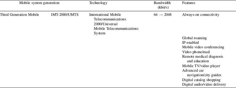
Apart from these hardware modules, there will be one or more microprocessor/controller modules to control the whole system and to run the protocol software and various applications such as voice call, data call, audio player, game, and so on. These will be discussed in more details in the next chapters.

Further Reading

Das, S.K. (2000) Microwave Signals and Systems Engineering, Khanna Publishers, Delhi.

Haykin, S. (2005) Communication Systems, John Wiley & Sons Inc., Hoboke

Proakis, J.G. and Salehi, M. (2005) Fundamentals of Communication Systems, Pearson Prentice Hall, Englewood Cliffs, NJ.

Tse, D. and Viswanath, P. (2005) Fundamentals of Wireless Communication, Cambridge University Press, Cambridge.