
File Browser (blue), 3D Viewport (red), Image Editor (violet), Shader Editor (green), Outliner (orange) and Properties (yellow)
The Shader workspace is composed of six parts. The File Browser is in the top left of the workspace. The 3D Viewport is in LookDev Shading mode and located in the top center of the workspace. Outliner is located in the top right of the workspace. The Image Editor is located at the bottom left of the workspace. The Shader Editor is located at the bottom center of the workspace. Properties is located on the right side of the workspace.
You already know about Properties, Outliner, and 3D Viewport. Let’s discuss the File Browser, Image Editor, and Shader Editor.
File Browser
File browser is a common term in the computer world. You cannot explore your files without it. It’s the same in Blender. File Browser allows you to open your files—.blend files, textures, images, downloaded objects, or anything that you need to complete your project or scene.

File Browser: View (pink), Navigation (red), Create New Directory (green), Display Mode (brown), File Sorting (violet), Show Hidden Files (blue), File Filtering (light blue), File Path (yellow)
View has three submenus. Display Size is the size of the column in your file browser. Recursion is the level of searching. Area is the display screen.
Navigation is used for browsing folders.
Create New Directory helps you create a new folder directly from Blender when you want your file to be in a specific folder that isn’t available in the current path.
Display Mode helps you see the file in a view that is comfortable for you. It can be in thumbnail view, short-list view, or long-list view.
File Sorting and File Filtering help you easily find files. There are a lot of files and file types inside a folder. You can filter (e.g., make them all .blend files and list them alphabetically) to let you easily find what you’re looking for.
Show Hidden Files opens a hidden file. If it happens that any media or project that you use here is hidden, you made it hidden for some purpose.
File Path is where you can see the path of your file, as shown in Figure 4-2, or directly open your project. The folder with an arrow is for browsing your files.
Now, let’s move on to the Image Editor.
Image Editor
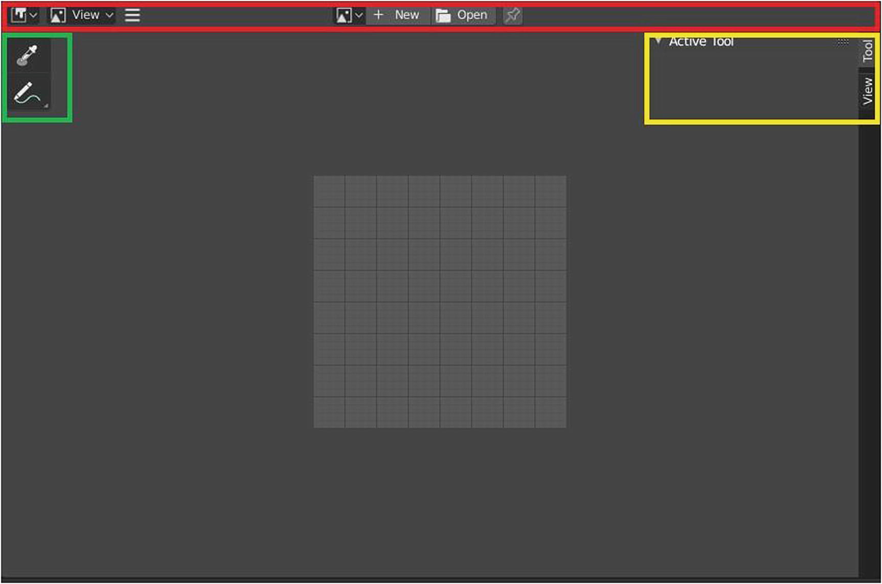
Image Editor header (top), sidebar (right) and toolbar (left)
By default, the toolbar (T) and the sidebar (N) are hidden. The big square at the center with grids in it is called Slot. This is where you see the image that you want to edit. You can save successive renders into the render buffer by selecting a new slot before rendering. If an image has been rendered to a slot, it can be viewed by selecting that slot.
In Header, there is View, New, and Open. This View Select menu has three different modes that you can choose in editing your image: View, Paint, and Mask.
In the Sidebar region, there is the Tools panel, where you can see your active tool, and the View panel, where you can have annotations.

Image Editor upon opening an image
As you can see in Figure 4-4, after we open an image, there are changes in the Header region as well as in the Sidebar region. There are four additional icons in the Header region; while in the Sidebar region, there are two additional panels.
I’d like to note that there are differences in the tool/command terms in the Image Editor (shown in the Shading workspace) and the Image Editor (shown in the Rendering workspace, which is covered in Chapter 5).
So, let’s discuss the Image Editor tools for the Shading workspace.
Tools
The shield icon in the Header region is called Fake User. It saves the current data-block, even it has no user; for example, the image we currently opened. Even it isn’t used as a material, it is saved for future use.
The icon next to it is New Image, which creates a new image. The folder icon is Open, which opens an image.
The X icon is Delete, which unlinks a data-block or the image. When you click it, the image disappears; you see again in the default Image Editor setup. If you accidentally delete something and want to bring it back without browsing the file once again, you need to click the image icon next to the File Search box, and there you can see the list of the images opened in the Image Editor. I’d like to note that even you use annotations here, when you delete the image, what you drew using the annotation remains. When you bring back an image after having changed its values in the Scope panel, the value is not reset.
In the toolbar, there is Sample, which picks sample pixel values under the cursor. The list of Annotate tools is always present: Annotate (2), Annotate Line (3), Annotate Polygon (4), and Annotate Eraser (5).
Now, let’s discuss the Sidebar region.
Sidebar
There are panels for tools, images, views, and scopes.
Tool Panel
The Tool panel features the settings for the active tool or the tool you’re currently using. Since Image Editor only has five tools, its settings aren’t complicated. The Draw tool allows you to see settings for the radius. It is the same for Annotate Eraser, but for Annotate, Annotate Line, and Annotate Polygon, what you can see in its setting are color and notes.

Image Editor ➤ Tool panel with Annotation
Image Panel
The Image panel’s settings contain the Source, which indicates where the image came from. The settings that follow depend on the options you choose in the source. There are four options available: Single, Image Sequence, Movie, and Generated.
If you choose Single Image, the settings available include a box in which you can see the file name and the exact location of your image.
Pack Image, sitting at the left side of file name, packs an image as an embedded data in the blend file.
The Open/Accept button, the folder icon beside the file name, opens or browses the image in the file directory.
The Reload Image (Alt+R) button beside the Open/Accept button, reloads the current image from the disk.
Color Space indicates the color space in the image file to convert to and from when saving and loading the image. There are seven options: sRGB, Filmic Log, Linear, Linear ACES, Non-Color, Raw, and XYZ.
Alpha is the representation of alpha in the image file. There are four options: Straight, Premultiplied, Channel Packed, and None.
View as Render renders part of the display transformation.
Meta Data is the code data of the image.

The original image shown in Figure 4-6 is not yet imported in Blender 3D. As you can see, Non-Color, Raw, sRGB, and the original, which is in RGB, do not seem to have any differences, unlike what you can see in Filmic Log, Linear, Linear ACES, and XYZ.
First, what is Color Space? Once upon a time, human met the machine. Human wanted to create art with the machine but the machine couldn’t understand human language. One day, human found a way to break this boundary. Since machine could understand numbers and human was a genius in math, they created a number to represent each color. Red = 0%, Green = 0%, Blue = 0% means Black. Red = 100%, Green = 100%, Blue = 100% means White. Red = 100%, Green = 100%, Blue = 0% means Yellow. This is called color space . In other words, color space is the mathematical expression of color for the machine to understand it.
sRGB, Non-Color, Raw, Filmic Log, Linear, Linear ACES, and XYZ are the mapping of colors, created for digital purposes. To have a standard way of dealing with colors, sRGB was created by Microsoft and HP and is said to be the standard way of communicating with colors in many digital forms.
So now, let’s go back to the Image panel settings for Image Editor.
When you are in Filmic Log, Linear, Linear ACES, or sRGB, the Alpha setting is enabled, but when you are in Non-Color and Raw, it is disabled.
When the Source is set to Image Sequence, the setting is the same in Single Image. In Image Sequence, Frames indicates the number of images to use in a movie. Start, sets the global starting frame of the movie or sequence, assuming the first picture is numbered 1. Offset offsets the number frames in the animation. Cyclic cycles the images in the movie. Auto Refresh, which is enabled by default, refreshes an image on frame changes.
Image Sequence is used in animation and movie clips. In Source, the Movie option has the same settings as Image Sequence but includes Deinterlace, which deinterlaces a movie file on load.
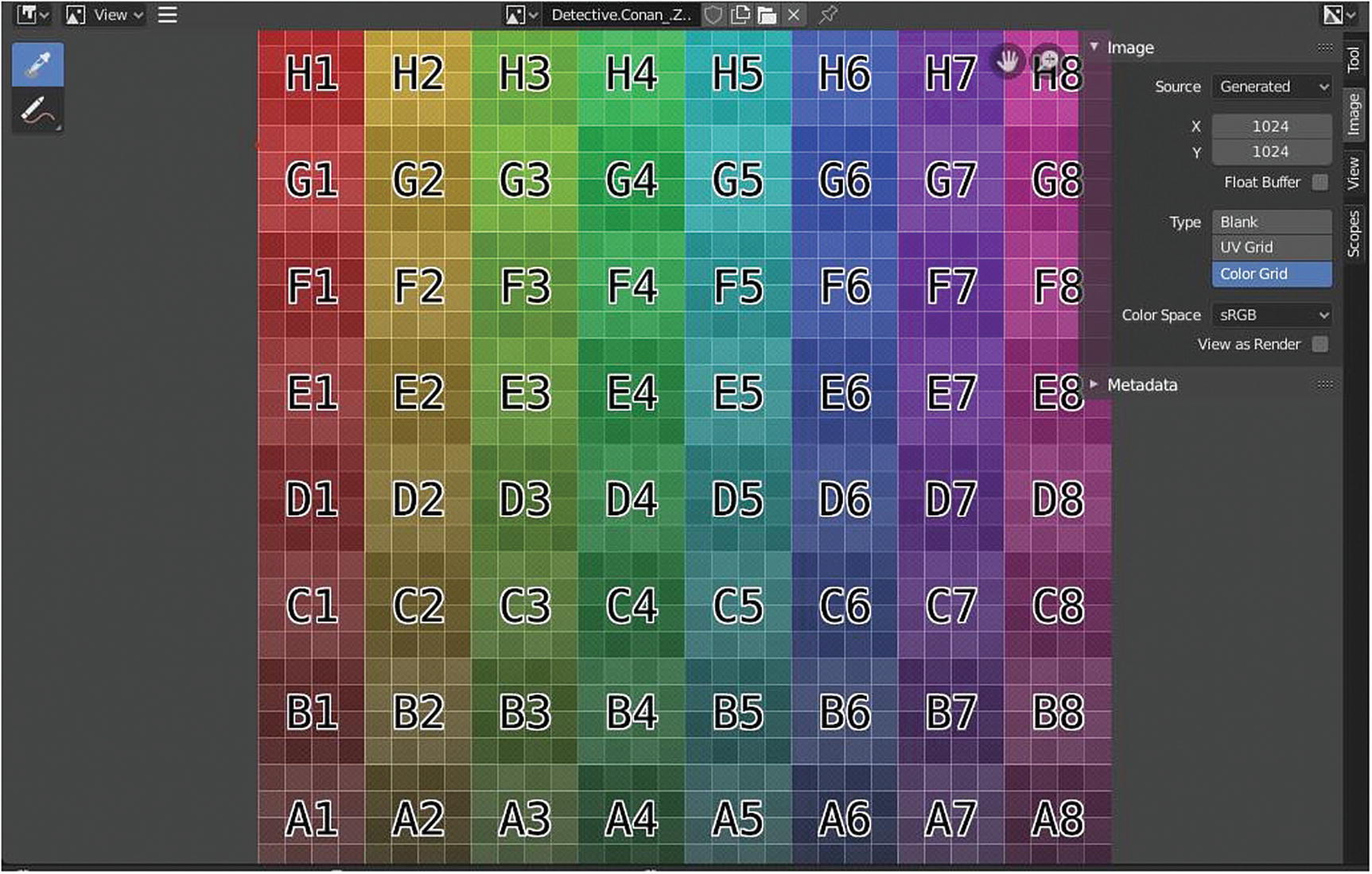
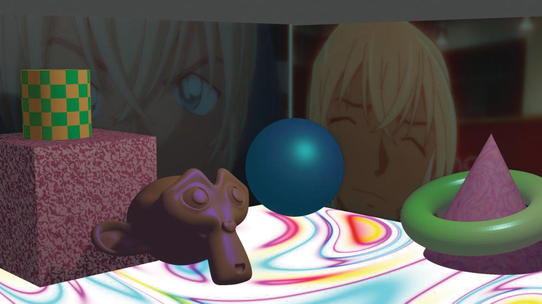
What happened to the two anime characters? When the source is in Generated, it converts the image into blocks of color. Its settings are quite different, as you can see in Figure 4-7. It has X/Y, which indicates the generated size of an image. Float Buffer generates a floating-point buffer. Type allows you to choose the generated image type. Blank leaves the slot blank. UV Grid makes it looks like a colored plus sign in a line in the slot. Color Grid is shown in Figure 4-7. It also offers Color Space and View in Render, which is enabled by default.
I’d like to note that when you select Generated and you go back to Single Image, you will not see your image in the slot—even if it is opened in the Header region. If you open it from the image list, you will not see it. In the settings, there is a notification that it can’t load the image, which is because Generated generates another image from the current opened image. It replaces it in the saved list in the Blender cache but it does not replace the file in your disk. If you want to use the original file, the best solution is to reopen the image with the Open/Accept button.

View panel
As you can see in Figure 4-8, the View panel’s settings are simple, just like the Tool panel. The Aspect Ratio X/Y displays the aspect. Repeat Image displays the image repeatedly outside of the main view. Annotation allows you to see the color of the note, the thickness of the annotate tool, and to delete and add notes.
The Scope panel has five setting: Histogram, Waveform, Vectorscope, Sample Line, and Sample.
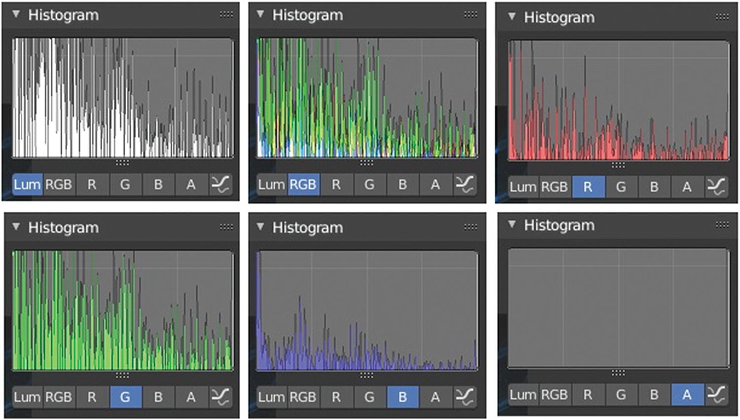
Scope panel ➤ Histogram
Figure 4-9 shows that there is a lot of green in my image but little blue. A luma represents the brightness in an image.

Scope panel ➤ Waveform
Just like in the Histogram, you can see the color data of an image by category. Waveform displays luminance with IRE values. IRE represents the scale invented by the International Radio Engineers Society. Essentially, it is designed to match the capabilities of early televisions to display an image. Anything at 0 is completely black, with no detail, and anything above 100 is clipped and white, with no detail.
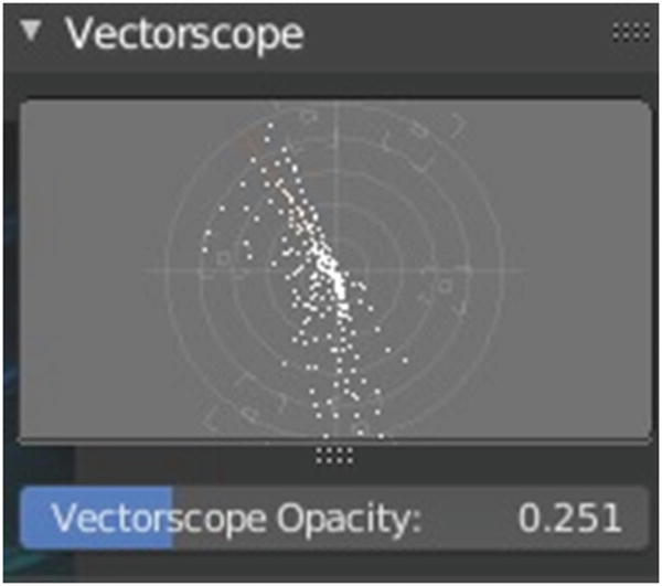
Scope panel ➤ Vectorscope
Vectorscope shows the hue and saturation. It displays six color targets fixed into an odd-shaped pattern on a grid. In fact, each color is represented by two targets; but what is important about the vectorscope is that it displays color information that the waveform monitor does not.
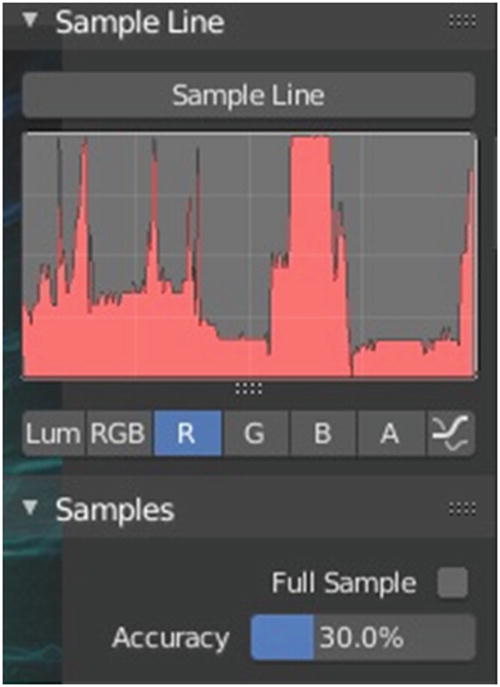
Scope panel ➤ Vectorscope
These two settings get a color data sample from a particular part of an image. When you click the sample line, it creates a line for you to select the part of the image to determine the luma content in it. Full Sample samples every pixel of the image. Accuracy sets the proportion of the original image’s source pixel lines to the sample.
Learning scopes can help you get the right balance of color for your project, that’s why it is important. We cannot see easily see its effect since it comes with the right combination of adjustments.
This is the end of the discussion on Image Editor. Let’s now proceed to the Shader Editor.
Shader Editor
The Shader Editor is where you can create amazing materials using the combination of different nodes. You can also edit materials that are used in Cycles and the Eevee render engine. Materials, lights, and backgrounds are all defined using a network of shading nodes. These nodes output values, vectors, colors, and shaders.
This editor is composed of a header region, a toolbar (T), a sidebar (N), and a node editor.
Header

On the left side, there is the Select menu for the Editor Type and the Shade Type. The View menu consists of commands for viewing the toolbar and sidebar, zooming in/out, viewing selected/all, and different options in the view area. The Select menu consists of various commands for selecting things. The Add menu adds nodes, which you can do by holding Shift+A in the Node Editor section. The Node menu consists of commands for working with nodes.
Use Nodes enables the shader nodes to render the material. Slot selects active material for your project. You can also see the materials you already created for a specific object. There are the Fake User, New Material, and Delete buttons. The Pin Button keeps the current material selection fixed. There is also an arrow icon at the right side of the Header region pointing upward. This is the Parent Node Tree, which is used to go to the parent node tree. It is useful when you already have a lot of nodes, and you group and link node groups. The Snap Node Element consists of four options: Grid, Node X, Node Y, and Node X/Y.
Toolbar
Now, let’s proceed to the toolbar. If you press T, the toolbar will appear. It consists of the Select tool (W) for single selection, Box Select (B) for box selection, Circle Select (C) for circle selection, the Lasso tool (L) for lasso selection, Annotate (D/3) for creating annotations, Annotate Line (3/4) for creating a line note, Annotate Polygon (4/5) for creating a polygon note, Annotate Eraser (5/6) for erasing annotations, and Links Cut (6/7) for cutting links.
Note
Once again, the default hotkey for Annotation is D, but when you click any annotation tool, its hotkey changes. In this toolbar, the D is replaced by 3. This affects other tools’ hotkeys. Be aware of those changes.
Node Editor
The Node Editor is where you edit or create the materials. There are a lot of materials, set by category; it depends on the render engine that you use.
When it comes to the Materials menu under the Input, Texture, Color, Vector, Script, Group, and Layout categories, the three render engines—Eevee, Cycles, and Workbench—have the same list; whereas in the Converter, Output, and Shader categories, there are differences. I won’t say much about the Input and Output categories. There are several options, all of which are fairly straightforward.

Sockets
The sockets that are placed on the right side of the nodes are called output sockets. The sockets placed on the left side are called the input sockets. These sockets are responsible for linking the nodes and transmitting information from one node to another.
Next, I discuss some of the nodes a bit.
Principled BSDF
Principled BSDF combines multiple layers into an easy-to-use node. It is based on the Disney principled model also known as a PBR shader. Image textures painted or baked from software like Substance Painter may be likely linked to the corresponding parameters in this shader.
Base Color sets the diffuse/metal surface color.
Subsurface sets the value for mixing the base color and subsurface color.
Subsurface Radius sets the average distance that light scatters below the surface.
Subsurface Color sets the subsurface scattering color.
Metallic sets the Metallic value.
Specular sets the dielectric specular reflection value.
Specular tint sets the value of tints facing the specular reflection using the base color while glancing reflection remains white.
Roughness sets the roughness value.
Anisotropic sets the amount of anisotropy for specular reflection.
Anisotropic Rotation rotates the direction of the anisotropy.
Sheen sets the amount of soft velvet like reflection near edges.
Sheen Tint mixes the white and base color for sheen reflection.
Clear Coat sets extra white specular layer on top of others.
Clear Coat Roughness sets roughness of clearcoat specular.
IOR sets the index of refraction value.
Transmission mixes between fully opaque surface at zero and fully glass like transmission at one.
Transmission Roughness controls roughness used for transmitted light with GGX distribution.
Emission lights emission from the surface.
Alpha controls the transparency of the surface of the surface.
Normal controls the normals of the base layers.
Clearcoat Normal controls the normals of the Clearcoat layer.
Tangent controls the tangent for the Anisotropic layer.
There are also Distribution properties. GGX is less physically accurate but faster than multiple-scattering GGX and enables Transmission Roughness input. Multiple-Scattering GGX provides energy-conserving results that would otherwise be visible as excessive darkening and takes multiple bounces or scattering events between microfacets into account. Subsurface Method: Christensen-Burley is an approximation of physically-based volume scattering; it gives less blurry results than the Cubic and Gaussian functions. Random Walk provides the most accurate results for thin and curved objects.
Mix Shader
Mix Shader mixes shaders together. Mixing can be used for material layering. Factor input is for nodes that enhance the mixing of shaders, like Layer Weight.
Diffuse BSDF
Diffuse BSDF adds Lambertian or Oren-Nayar diffuse reflection. It has Color input, Roughness input, and Normal input.
Glossy BSDF
Glossy BSDF adds reflections with microfacet distribution; it is mostly used for materials like mirrors and metals.
Emission
Emission adds the Lambertian emission shader. It can be used as a light since it has a luminance effect.
Subsurface Scattering
Subsurface Scattering adds subsurface multiple scattering for materials such as skin, wax, marble, milk, and so forth. Rather than light being reflected off the surface, it penetrates the surface and bounces around internally before being absorbed or leaving the surface at a nearby point.
Image Texture
Image Texture adds an image file as a texture.
Math is part of Converter and performs math operations.
Mapping is part of Vector and transforms an image or procedural textures. You can use this to move, rotate, or scale textures when you connected it to Image Texture.
Texture Coordinate is part of Input and commonly used for the coordinates of textures, typically used as inputs for the vector input for texture nodes.
Mix Node or MixRGB is part of Color and mixes images by working on the individual and corresponding pixels of the two inputs.
Color Ramp is part of Converter and maps values to colors with a gradient.
Fresnel is part of Input and computes how much light is reflected off a layer, and where the rest will be refracted through the layer.
Material Output outputs surface material information to a surface object.
Light Output outputs light information to a light object.
World Output outputs light color information to a scene’s world.
Let’s now proceed to a sample project. It is best to discuss with examples.
Sample Project
We will not use the Suzanne project this time. You can use a scene that you made, just like the other scenes.
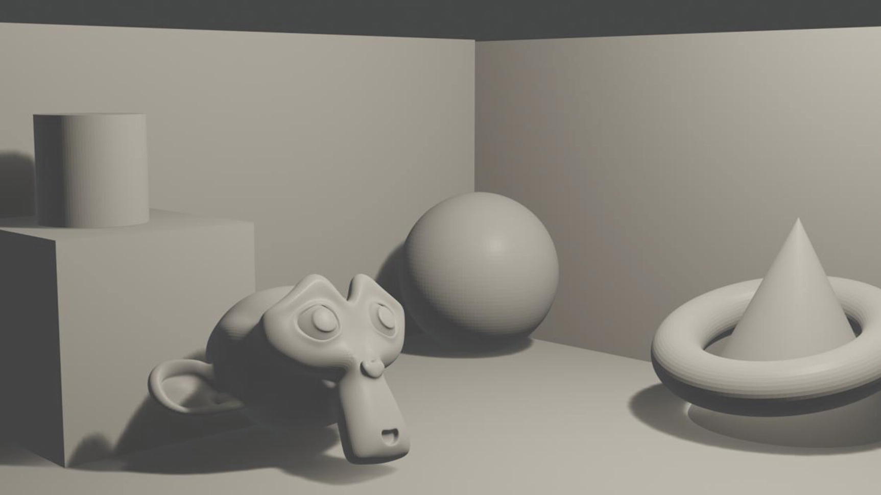
Rendered scene in Eevee
Simple, right? Yes. Let’s just do a simple project for this example. All of the examples are rendered in Eevee.
First, I applied a modifier to the Suzanne mesh and sphere but not to the torus, cone, and cylinder. I adjusted their vertices in the mesh pop-up menu settings that only appear when you add mesh. So, it’s better for you to decide how many vertices that you plan to use beforehand.
- 1.
In the Layout workspace, click the plane on the left side.
- 2.
Go to the Material panel in Properties and click New.
- 3.
Go to Subsurface Color and click Image Texture. The settings include a drop-down of the images opened in Blender, a button for creating new image, a button for browsing images on your drive, a drop-down list for setting texture interpolation, a drop-down list for projecting a 2D image on an object with a 3D vector, and a drop-down list for how the image is extrapolated past its original bounds.
- 4.
Open an image on your drive. Figure 4-16 shows what happens.

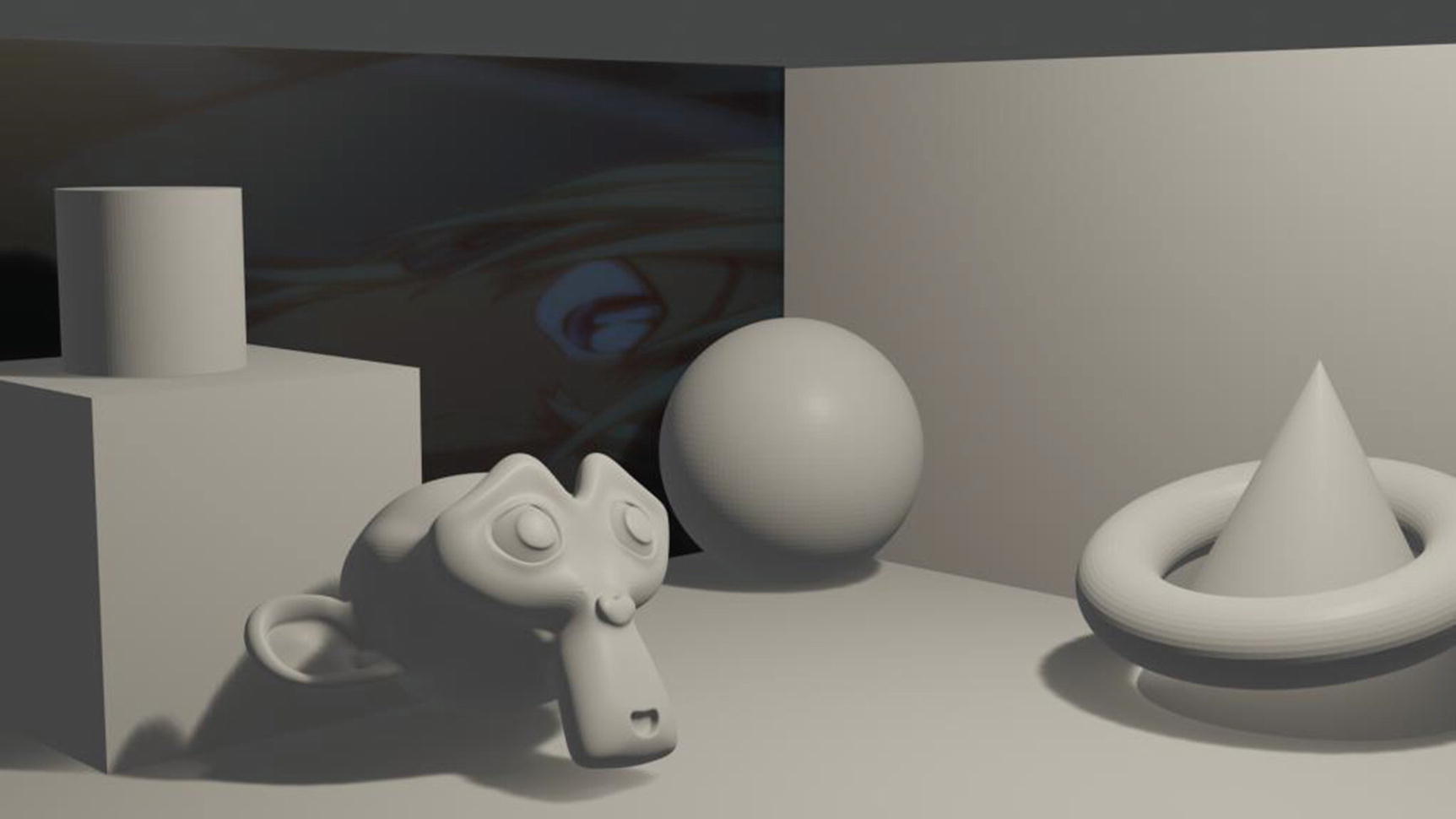
Rendered Scene in Eevee after Applying Image Texture in Layout workspace
No, no, no. That picture is not an editorial mistake. It’s really a result of Image Texture for now cause we still not doing one thing to implement this completely, the UV mapping.
UV mapping is a method for translating a 2D image into a 3D object. Well, here’s a better explanation: if you want to wrap a present, how do you do it? Our gift wrapper is a plain flat square object. You can think of a gift wrapper as a 2D image. Think of things like a tumbler, plate, cup, and other things around you as 3D objects. When you apply an image texture, you need to wrap it around the 3D object; that’s why we have a UV editing workspace. Unfortunately, this subject is not discussed much in this book because it’s a bit advanced.
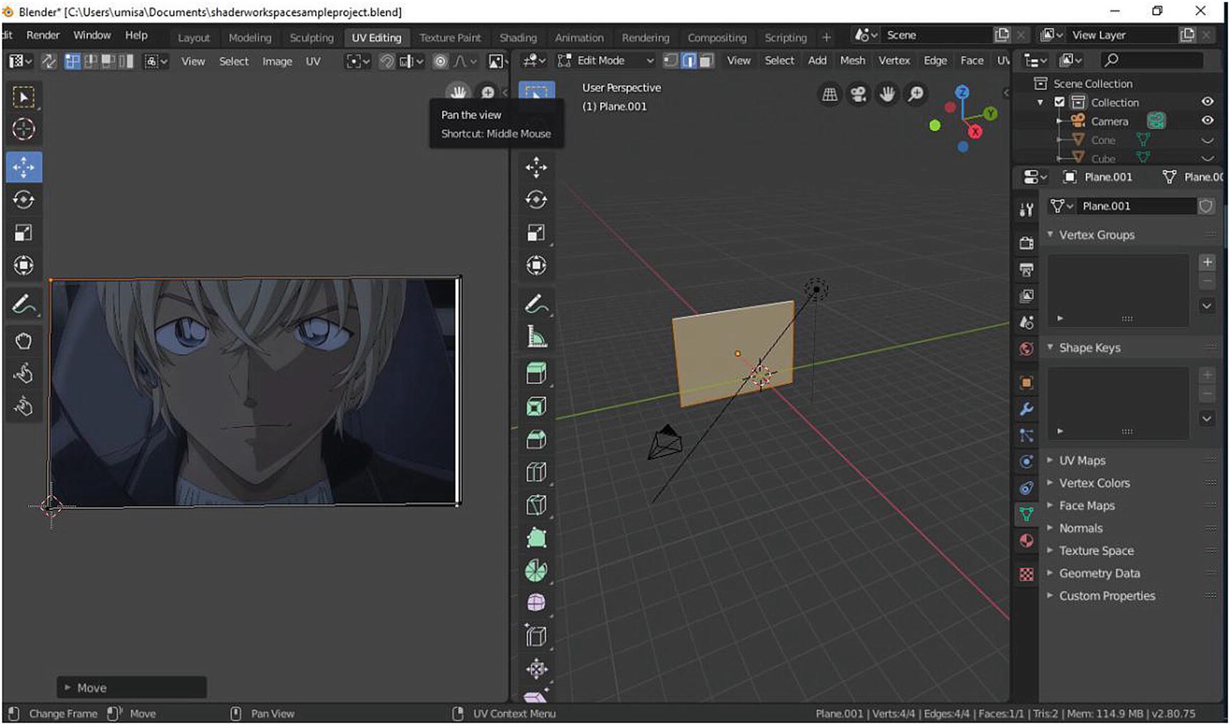
So, now, let’s go back to our project. Since you’re only going to use Image Texture on the plane, it’s easy to wrap it up. Go to the UV Editing workspace, and if you already see your image in the UV editor on the left side of your screen, that’s it! But when it comes to very detailed things, this becomes more complicated.


Rendered result with Image Texture and UV Unwrapping
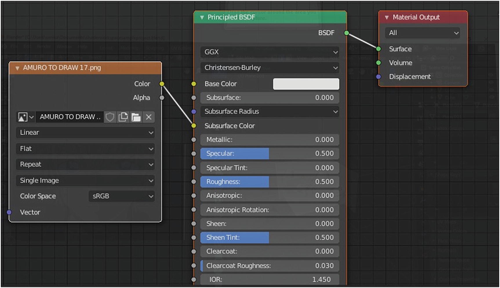
Nodes set up in the Shading workspace
Rendered result of the setting Subsurface to 1
It’s already there but wait, the picture is not in the right position. Go back to the UV editor. When you have a texture image, you see white lines around it, which represents the seam or the image placement of the object when 3D is cut to 2D. Select it all and rotate it. Adjust it until you get the result that you want.
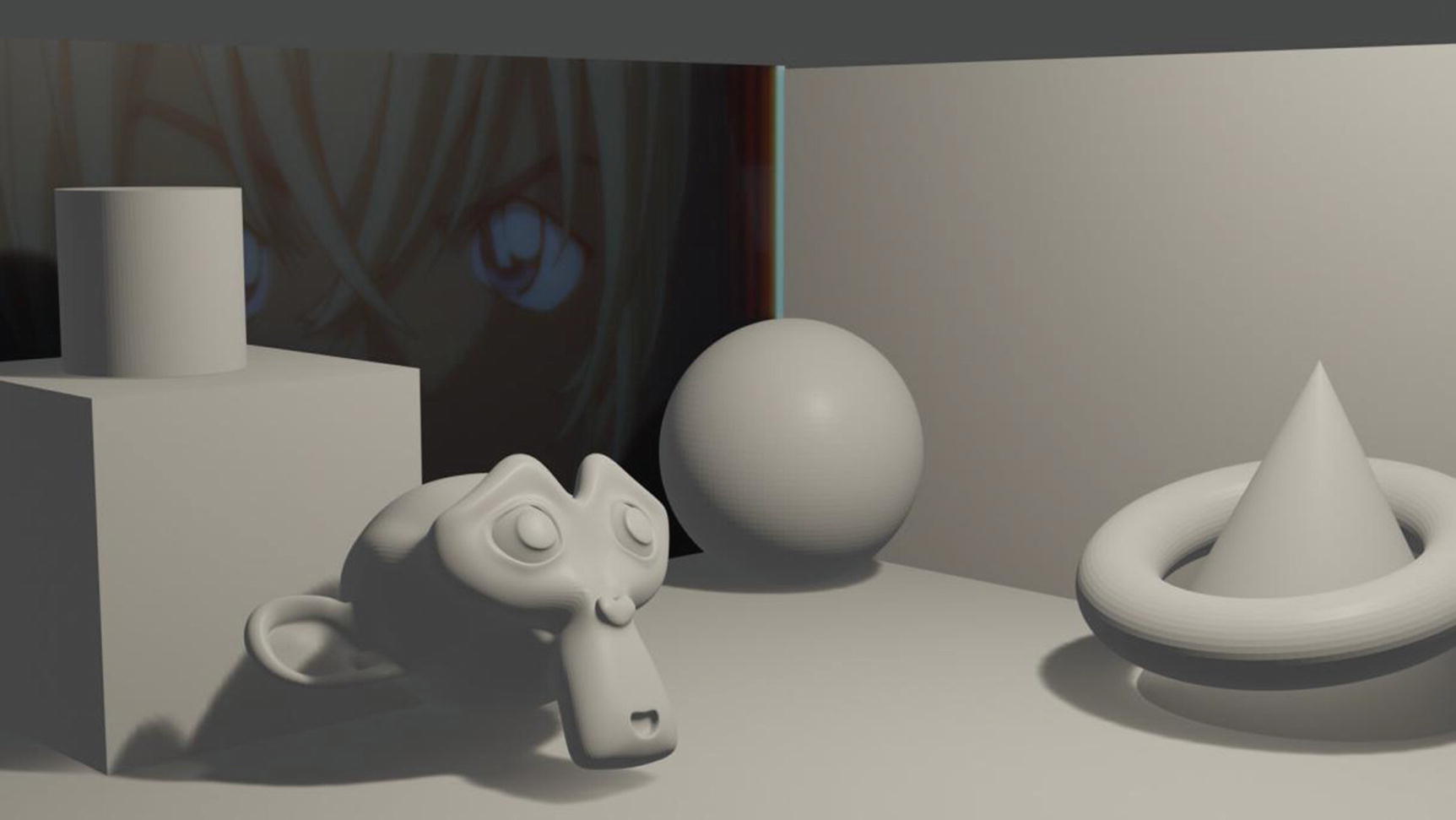
New render result
Try to add an image texture in the plane on the right side, but instead of using UV editing for positioning the image, use the Mapping node, which is part of the Vector category, and the Texture Coordinate node, which is part of the Input category.
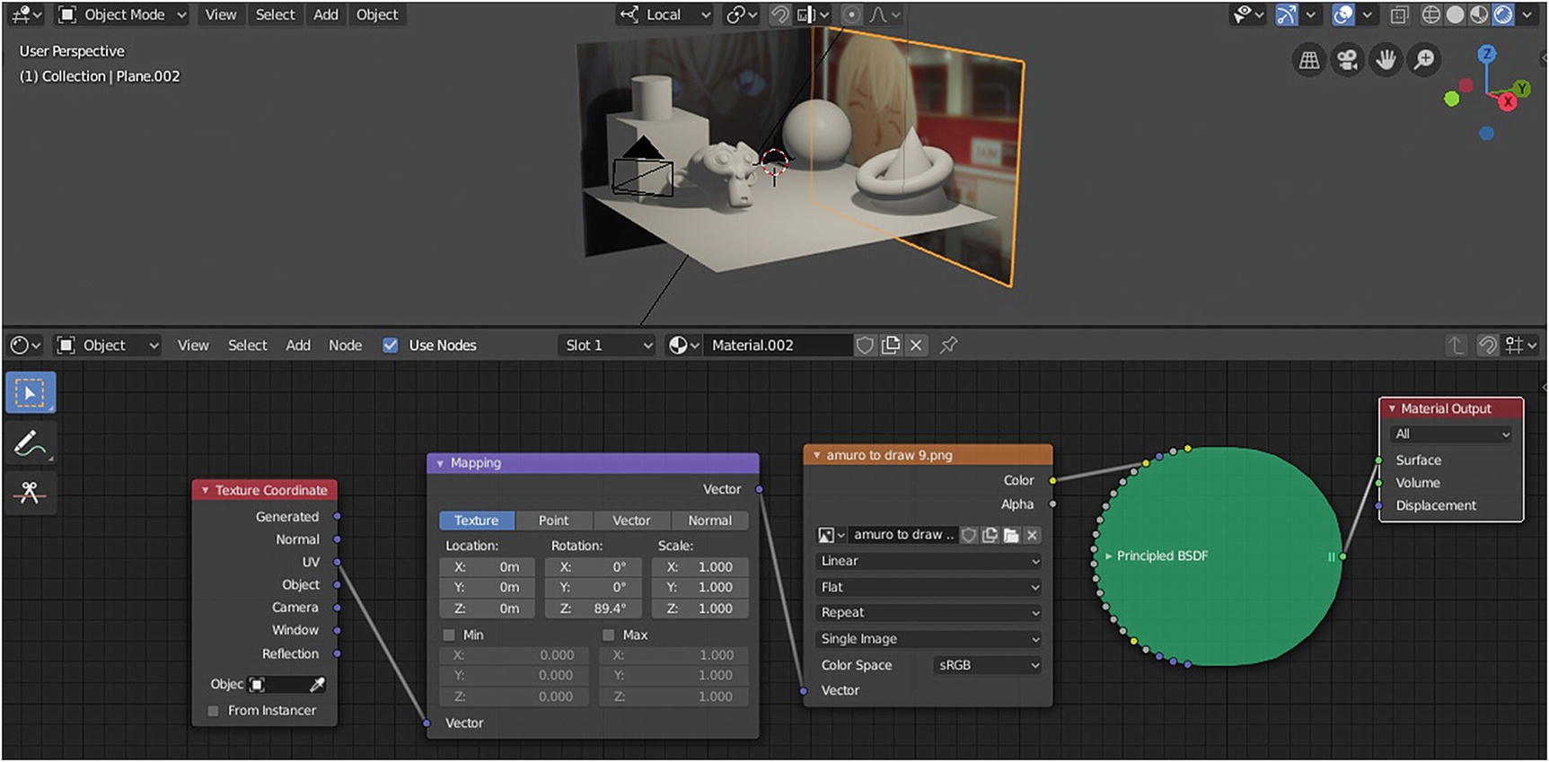
Nodes setting for the right plane
Choose the texture, which is commonly used when using Mapping for image textures, and set the Z rotation to 89.4 degrees. As you can see in the 3D Viewportat the top, it was already in the desired position. When it was imported, it was in the reversed position. This is like a transformation tool for an image texture. You need to link Mapping to Texture Coordinate’s UV output because your basis is the UV of the image texture.
Generated automatically generates texture coordinates from the vertex positions of the mesh without deformation, sticking them to the surface under animation. Normal is the normal object space. Object is the object as a source for the coordinates. Camera positions the coordinates in the camera space. Window locates the shading point on the screen. Reflection is the direction of the reflection vector as a coordinate.
You might notice that your Principled BSDF shape became oblong. You can see the small triangle in the header of the node. When you click it, it turns the node into an oblong shape. This can be helpful when you want to minimize the space occupied by your node shader.
For the plane in the bottom, delete the Principled BSDF in the node editor and replace it with Emission Shader. You should also add Magic Texture, which adds a psychedelic color texture. I use it to add effects on my materials when I use plain colors.
Operation is set to Logarithm.
Value 1 is set to 0.500.
Value 2 is set to 0.300.
Operation is set to Add.
Value 1 is set to 2.100.
Value 2 is set to 0.100.

Nodes settings for the bottom plane
You see the effect of our node setup in the bottom plane. Without Magic Texture and the math node, it was only a plain color. If you remember, you used emission in the Text object in the Suzanne project, and it was plain green. That’s only an Emission effect because it is a shader that can be used as a light object. So, unless you connect it with textures and so forth, it will only emit a plain color.
- 1.
Delete the Principled BSDF and replace it with Diffuse BSDF.
- 2.
Add Glass BSDF and combine the two using the Mix Shader.
- 3.
Add Fresnel node and connect it to Glass BSDF.
- 4.
Set the Diffuse color to E7B354 and Roughness to 0.438.
- 5.
Set the Glass BSDF color to 4907FF, Roughness to 0.508, and Properties to Beckmann.
- 6.
The Fresnel set the IOR to 4.950.
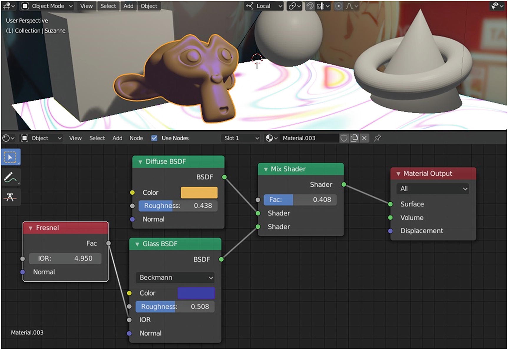
Nodes setting for the Suzanne mesh

Nodes in groups
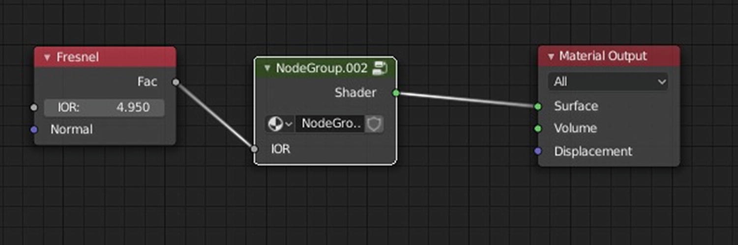
Node setting outside the group
To ungroup the materials, you need to click the node group. Then go to Node menu ➤ Ungroup or hold Ctrl+Alt+G. To make a group, you need to select the nodes you want to include in the group, then go to Node menu ➤ Make group or press Ctrl+G.
Diffuse color: 0C0FC9 and Diffuse Roughness: 0
Glossy BSDF color: 00E720, Glossy BSDF Properties: GGX and Glossy BSDF Roughness: 0.500
ColorRamp Properties: RGB and Linear, ColorRamp Color: FC0500 and 00B3FF, Color Ramp Pos: 1 and Color Ramp Factor: 0.400
Wave Texture Properties: Bands and Sine, Wave Texture Scale: 7.000, Wave Texture Distortion: 24.700, Wave Texture Detail: 12.300, and Wave Texture Detail Scale: 3.400
Wave Texture adds procedural bands or rings with noise distortion, but personally, I like Magic texture. I use it to add an effect when I think that the shaders are plain.
Diffuse BSDF color set to 0C0FC9
Diffuse BSDF’s roughness set to 0.700
Glossy BSDF color set to 22DAE7
Glossy BSDF roughness set to 0.492
Mix Properties set to Multiple
Mix Factor set to 0.567
Mix Color1 set to 4567FF
Mix Color2 set to FF2117
Diffuse BSDF with a setting of 0018FF for color
Diffuse BSDF with a setting of E73575 for color
Diffuse BSDF with a setting of E7E7E7
Add Shader that connects the last two Diffuse Shaders
Mix Shader that connects the first Diffuse BSDF to the Add Shader and with a setting of 0.683 in Factor
Noise Texture that connects to the color of the third Diffuse BSDF and with a setting of 7.500 in Detail and 10.600 for Distortion
Math node with a setting of Add in properties: 4.500 for the first value and 0.300 for the second
For the cylinder mesh, I suggest the Checker texture. For the torus mesh, the Specular node and Diffuse Shader and mix its value with Mix Shader. Connect the RGB Curves to the Base Color of the Specular Node input and Diffuse BSDF Color input. Also add Gradient texture and connect it to the RGB curves input.
Note
Yes, I do love to apply texture nodes to make my shader nodes interesting.

Node settings for cube mesh (upper image), sphere mesh (center image), and cone mesh (bottom image)
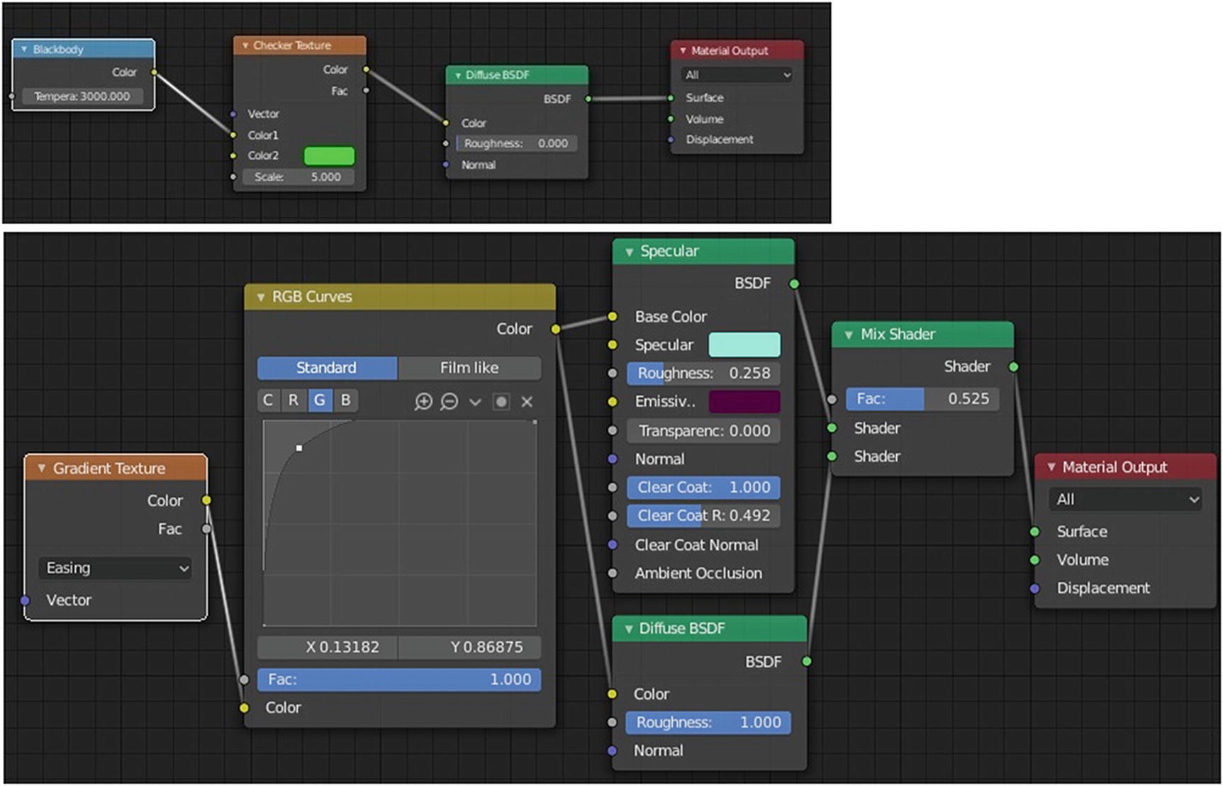
Node setting for cylinder mesh (top) and torus mesh (bottom)
Rendered Result
You can adjust the strength of emission to 20 to see more details. I’d like to note, once again, that this is rendered from Eevee.