I talked about the Blender user interface in Chapter 1. I talked about the Layout workspace, Modeling workspace, and Shader workspace in Chapters 2, 3, and 4. You even had a sneak peek of the UV editing workspace and many Blender features through sample projects. I also discussed the fundamentals of light and color and the various editors.
The focus of this chapter is the Animation workspace and the Rendering workspace. So, let’s start the tour!
Note
As animation is harder to demonstrate on the page, I have not provided sample projects for every topic in this chapter. You’ll see plenty of options along the way to allow you to use Blender for your own animations.
Animation Workspace
This workspace is where you can create and edit your animation. This workspace contains 3D Viewport, Outliner, Properties, Dope Sheet, and Timeline.

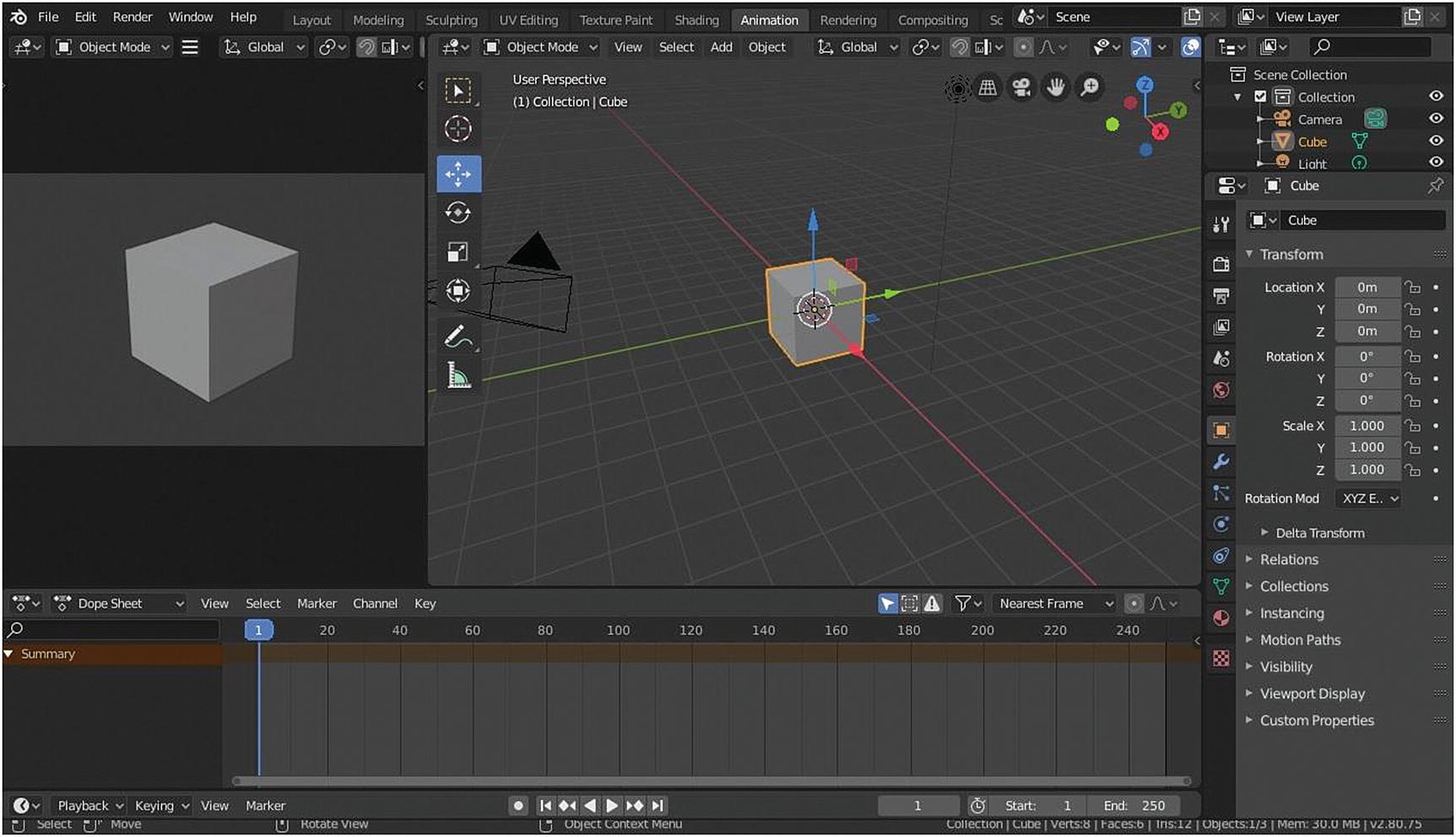
Animation workspace
Figure 5-1 shows the 3D Viewports. One is in camera perspective, which you can see by pressing 0 in your numpad or by selecting View ➤ Viewpoint ➤ Camera. The other viewport is in its regular settings.
Dope Sheet
Dope Sheets give the animator a bird’s-eye view of the keyframes inside the scene. This is inspired by the classical hand-drawn animation process, in which animators use charts, showing exactly when each drawing, sound, and camera move will occur, and for how long. This is also called an exposure sheet.
Dope Sheet is divided into three regions: Header region, Channel region, and Main region. It has six modes: Dope Sheet, Action Editor, Shake Key Editor, Grease Pencil, Mask, and Cache File.
Dope Sheet ➤ Dope Sheet Mode

Dope Sheet mode
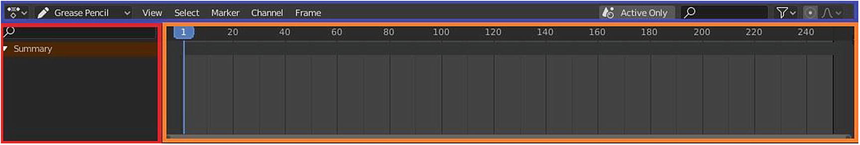
The one in inside the blue rectangle, place in the top, is the Header region. The one on the left is the Channel region, and the one on the right is the Main region. It also has a sidebar, but it is hidden by default; you can access it by pressing N on your keyboard.
Let’s discuss the Header region. On the left is the Select menu for Editor Type. Next to it is the Select menu for Dope Sheet mode. Next are the Header menus, which are View, Select, Marker, Channel, and Key. Then, there are three icons for filtering. Only Selected (arrow icon) is for showing/including only the channels related to selected objects and data. Display Hidden (small dotted square) is for showing/including the channels from objects or bones that are not visible Show Errors (exclamation point inside a triangle) is for showing/including F-curves and drivers that are disabled or have errors.

For example, you wanted to animate those three arrows. To animate, elements called Keyframes allow you to tell the software, “This is how big the arrow is. This is where the arrow is at this moment.” But there is a problem. If I want to make a too big arrow to medium arrow, then too small arrow, will I repeatedly assign keyframes? I use keyframes to indicate the movement of my animation. This is where the F-curves come in. When you create set a keyframe from one end to another to create an animation, it creates an F-curves or a line that you can move for an effect for your animation. This helps you lessen your efforts with repeatedly creating keyframes and from preventing multiple keyframes. Let’s go back to the Header region.
Frame defines increments on the Timeline/Dope Sheet/Graph Editor. The number, seconds, and so forth. The part of the timeline where your animation runs is the frame. Think of it as a time frame. That is the time frame that you allotted your animation. Remember, we can assign or set where the frame will start and end through the playback pop-over menu.
Keyframe is a frame where a change occurs in the Timeline/Dope Sheet/Graph Editor. It’s an indication that changes happen in this part of frame. F-curves lessen the usage of keyframes.
Let’s go back to the traditional animation. The animation where animators use paper and they flip it to perform an action for you to easily imagine this part. If you have the whole pad of paper, think of it as the frame. Since it is traditional, paper and pencil are used, think of the paper as the keyframes. Imagine how many times you need to move, re-create you object, move a small detail to have a single object animate. It cost you a lot when doing it. That’s why when animation are digitized, in 2D animation they create this so called Motion Tween that links two key frame that is apart. You need to create a big circle and insert a keyframe then leave frames apart insert another keyframe where you draw a small circle and you will see when you play it, it automatically animate the big circle turning to small circle. Magic? Well, the magic of math and technology. This Motion Tween is the same as F-Curves.
Let’s go back to the Dope Sheet Header region.

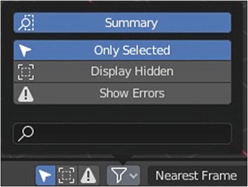
Filters
From the top, there is Summary, which is enabled by default. This is the summary in the Channel region. Only Selected is enabled by default. Next are Display Hidden and Show Errors. As you can see, these settings are for enabling/disabling or showing/hiding element. In Show Errors is a search box called Name Filters. This name filters can be seen also in Channel region. In these settings are the Filter Types. This filter types help you choose what to include in visualization related to animation data.
Next is the Select menu for the snapping tool. There are six options. No Auto Snap means no snapping at all. Frame Step means snap to 1.0 frame intervals. Second Step means snap to 1.0 second intervals. Nearest Frame means snap to actual frames. Nearest Second means snap to actual seconds. Nearest Marker means snap to nearest marker. By default, it is set to Nearest Frame.
Last is the Proportional Editing Falloff. There are eight options: Random, Constant, Linear, Sharp, Inverse Square, Root, Sphere, and Smooth.
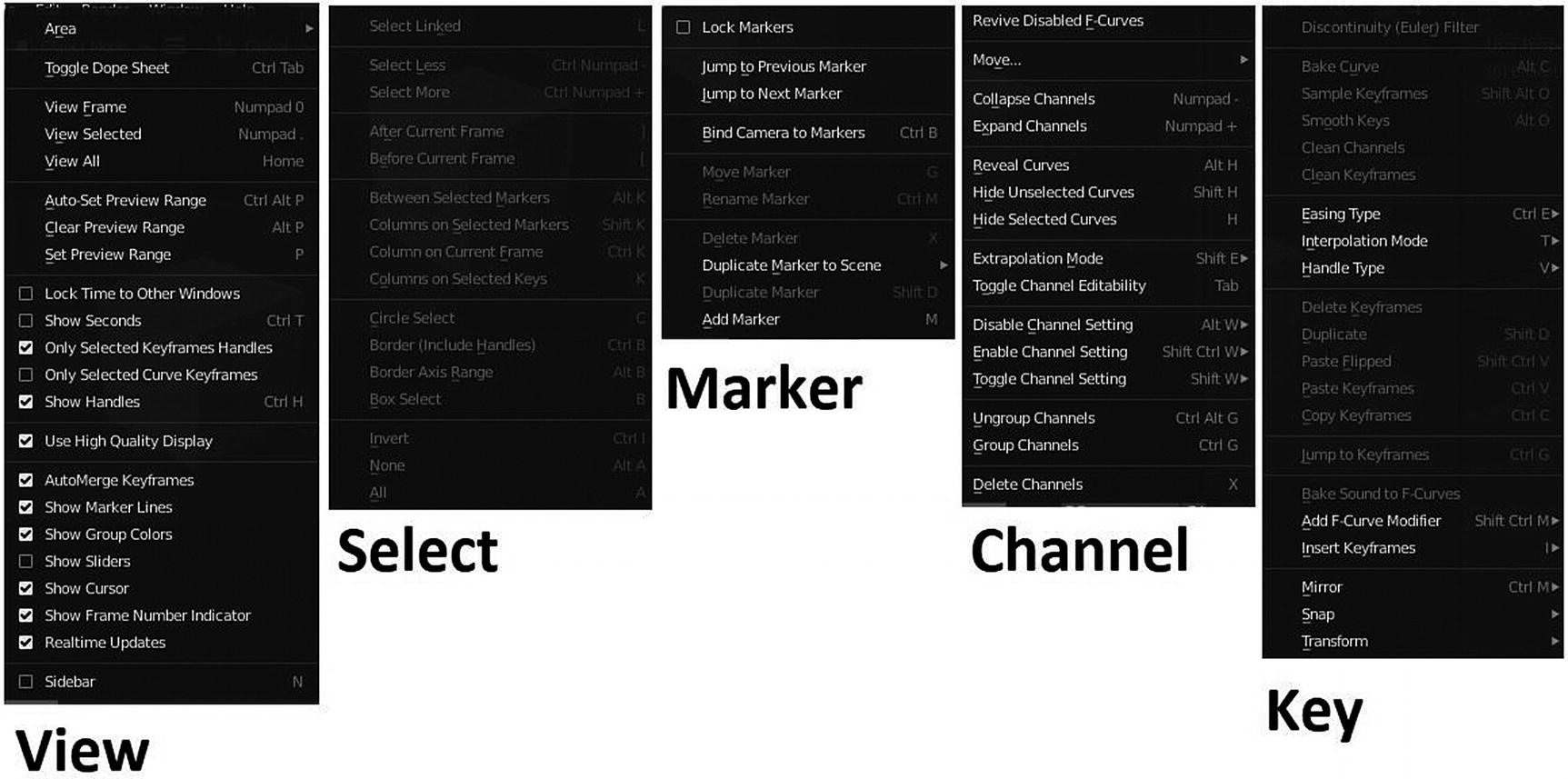
Dope Sheet Mode Header Menus
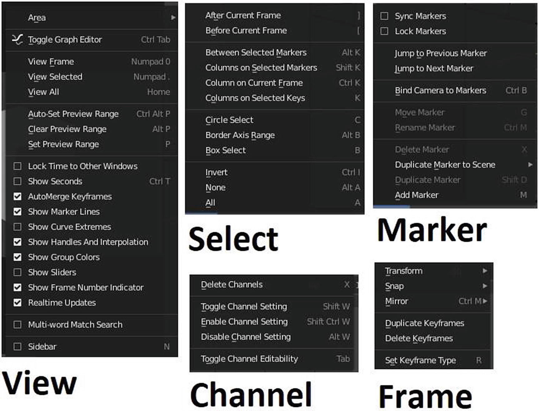
There is View, Select, Marker, Channel, and Key.

Figure 5-5 is taken when I still don’t have anything in the Dope Sheet. In the Marker menu, some commands are disabled. It’s because there are no markers in the Dope Sheet. Most Marker commands only work when your cursor is in the marker itself or when you hover your cursor to the marker, even when using shortcut keys.
The View and Select menus are very straightforward, so you can refer to Figure 5-5 for the hotkeys.
Markers Menu
What are Markers? What exactly its purpose? Markers denote frames with key points or significant events within an animation. Example, it could be that a character animation starts, the camera changes position, lighting on change it color or a cube moves it position. Markers can be given names to make them more meaningful at a quick glance. Unlike keyframes, markers are always placed at a whole framed number. You cannot set a marker at frame 2.5.
Let’s discuss what’s in the Markers menu. Sync Markers syncs markers with keyframe edits. Lock Markers prevents marker editing. Jump To Previous Markers jumps to previous marker from the current marker selected. Jump to Next Markers jumps to next marker from the current marker selected. Bind Camera to Markers (Ctrl+B) binds the selected camera to a marker on a current frame, and in this way, the operator allows markers to set the active object as the active camera. Move Markers (G) moves selected time marker. Rename Markers (Ctrl+M) renames first selected marker. Delete Markers (X) deletes selected time marker. Duplicate Marker to Scene copies selected marker to another scene. Duplicate Marker (Shift+D) duplicates selected marker and Add Marker (M) adds a new time marker.
Channel Menu
Let’s discuss the Channel menu. Revive Disabled F-Curves clears the disabled tag from all F-curves to get broken F-curves working again. Move rearranges selected animation channels. There are four options: To Top (Shift+Page Up), Up (Page Up), Down (Page Down), and To Bottom (Shift Page Down). Collapse Channel (Numpad-) collapses all selected expandable animation channels. Expand Channel (Numpad+) expands all selected expandable animation channels. Extrapolation mode sets extrapolation mode for selected F-curves. There are four options: Constant Extrapolation, Linear Extrapolation, Make Cyclic (F-Modifier), and Clear Cyclic (F-Modifier).
Let’s discuss Extrapolation mode. Extrapolation defines the behavior of a curve before the first and after the last keyframes. Constant Extrapolation is the default one. It curves before the first keyframe and the last one has a constant value. Linear Extrapolation has curved ends that are straight lines as defined by their first two keyframes (respectively, their last two keyframes). Make Cyclic and Clear Cyclic are for F-modifiers, which are similar to object modifiers, in that they add non-destructive effects, that can be adjusted at any time, and layered to create complex effects. This can be found when you are using Graph Editor.
In the Channel menu, we also have Toggle Channel Editability (Tab) toggles editability of selected channels. Disable Channel Setting (Alt+W) disables specified setting on all selected animation channels. There are two options: Protect and Mute. Enable Channel Setting (Shift+Ctrl+W) enables a specified setting on all selected animation channels. There are two options: Protect and Mute. Toggle Channel Setting (Shift+W) toggles specified setting on all selected animation channels. There are two options: Protect and Mute. Ungroup Channel (Ctrl+Alt+G) removes selected F-curves from their current groups. Group Channels (Ctrl+G) adds selected F-curves to a new group. Delete Channels (X) deletes all selection animation channels.
Key Menu
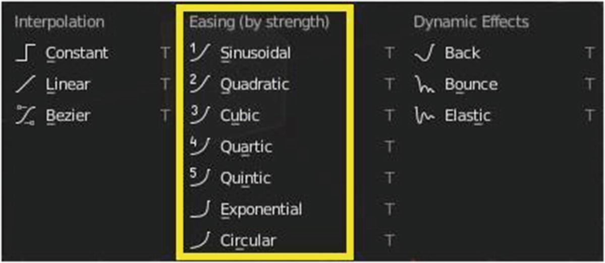
Let’s discuss the Key menu. Sample Keyframes (Shift+Alt+O) adds keyframes on every frame between the selected keyframes. Clean Channels/Clean Keyframes simplifies F-curves by removing closely spaced keyframes. Interpolation mode (T) sets the interpolation mode for the F-curve segments starting from the selected keyframes. There are 13 options divided into three categories. In Interpolation, there is Constant, Linear, and Bezier. In Easing, there is Sinusoidal, Quadratic, Cubic, Quartic, Quintic, Exponential, and Circular. In Dynamic Effects, there is Back, Bounce, and Elastic. Let’s discuss this a bit.
Constant means there is no interpolation at all. The curve holds the value of its last keyframe, giving a discrete curve. Usually only used during the initial blocking stage in pose-by-pose animation.
Linear is a simple interpolation creates a straight segment, giving a non-continuous line. It can be useful when using only two keyframes.
Bezier is the more powerful and useful interpolation, and the default one. It gives nicely smoothed curves.
Back is cubic easing with overshoot and settle. Use this one when you want a bit of an overshoot coming into the next keyframe, or perhaps for some wind-up anticipation.
Bounce is exponentially decaying parabolic bounce like when objects collide.
Elastic is exponentially decaying sine wave like an elastic band. This is like bending a stiff pole stuck to some surface, and watching it rebound and settle back to its original state.
The options under Easing are different methods for easing interpolations for F-curve segments. The Robert Penner Easing Equations are equations that define preset ways that one keyframe transitions to another, which reduce the amount of manual work, the inserting and tweaking keyframes, to achieve certain common effects.
The Easing is the transition from one key frame to the next. When you are in the Graph Editor and you added a keyframes, and changed the Easing options, the curves of the Graph Editor change pretty dramatically.
Graph Editor
Each of the Easing mode plays with the curve of a keyframe. Before the key, we called it Easing in, and after the key, we called it Easing Out.
Let’s talk a bit about the Easing (by Strength) options.
Intepolation mode Options
If you want to create reactive animations (like a fight scene), you can use these five modes.
Exponential moves into the realm of unrealistic acceleration. If you wanted to do a slow motion effect that gradually moves closer to some keyed action and they hits suddenly and all at once while Circular basically abandons easing in and teleports before easing out again. This is well beyond unrealistic. This is well beyond unrealistic, and so it can be used in all manner or cartoonish styles to make some incredibly quick movements. Just be mindful about this mode’s impact looking fake or weightless.
These modes affect the animation quite differently if your easing type is set to Ease Out or Ease In and Out. You can right-click in the Graph Editor or press Ctrl+E to change the Easing type.
I provide a site where you can found a live demo and link to an ebook that explains more about the options for Easing for you to learn more: http://robertpenner.com/easing/.
Next, let’s consider Handle Type (V), which sets type of handle for selected keyframe. There are five options: Free, Aligned, Vector, Automatic, and Auto Clamped. Free breaks handle tangents. Aligned handle maintain rotation when moved and curved tangent is maintained. Vector creates linear interpolation between keyframes. The linear segments remain if keyframe centers are moved. If handles are moved the handle becomes Free. Automatic keyframes are automatically interpolated. Auto Clamped auto handles clamped to not overshoot.
Using Keyframe Type (R) sets type of keyframe for the selected keyframe. There are five options: Keyframe, Breakdown, Moving, Hold Extreme, and Jitter. Keyframe (white/yellow diamond) is a normal keyframe. Breakdown (small cyan diamond) is the breakdown state; for example, transition between key poses. Moving Hold (dark gray/orange diamond) is a keyframe that adds a small amount of motion around a holding pose and in Dope Sheet, it also displays a bar between them. Extreme (big pink diamond) an extreme state or some other purpose as needed. Jitter (tiny green diamond) a filler or baked keyframe for keying on ones or some other purpose as needed.
By Times Over Current Frame flips times of selected keyframes using the current frame as the mirror line.
By Values over Value flips values of selected keyframes; for example, negative values becomes positive or vice versa.
By Times over First Selected Marker flips times of selected keyframes using the first selected marker as the reference point.
Current frame snaps selected keyframes to the current frame.
Nearest Frame snaps selected keyframes to the nearest frame.
Nearest Second snaps selected keyframes to the nearest second.
Nearest Marker snaps selected keyframes to the nearest marker.
Finally, Transform transforms selected items by mode type. There are four options. Move (G) moves a single keyframe. Extend (E) extends the time between two keys. Slide (Shift+T) slides selected keyframes. Scale (S) scales selected keyframes.
You will learn more about this through sample projects.
Dope Sheet ➤ Action Editor Mode
Action Editor is where you can define and control actions. It enables you to view and edit the f-Curve data-blocks you defined as Actions in the F-Curve Editor.
It gives you a slightly simplified view of the F-Curve data-blocks. The editor can list all Action data-blocks of an object at once.
Each Action data-block forms a top-level channel. Note that an object can have several constraints (one per animated constraint) and pose (for armatures, one per animated bone) F-curve data-blocks, and hence an action can have several of these channels.

Dope Editor ➤ Action Editor mode
The Channel region has few a differences in the Dope Sheet. The Summary isn’t shown in the Channel region here but the Name Filter is.
Action Editor mode ➤ Filters
Wait a minute. Summary is enabled. How come that it isn’t shown in the Channel region? It’s because it only shows when you already have animation or actions to edit.
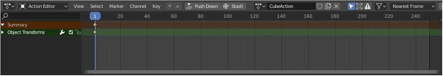
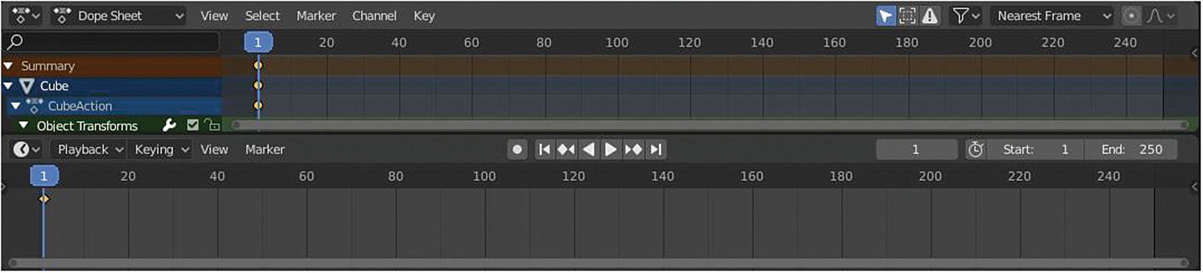
Action Editor mode ➤ Summary
See that after I add keyframes or simple animation, Summary appeared in the Channel region. The Header region has an up/down arrow. This is for switching to editing action in animation layer below or above the current action in the NLA stack. Next to it are the Push Down button and Stash button. Push down is to push action down on the NLA stack as a new strip while the Stash stores the selected action in the NLA stack as a non-contributing strip for later use. The up/down arrows, Push down, and Stash button are disabled since we’re not using the NLA or Non-Linear Animation Editor.
What is NLA? Non-Linear Animation (NLA) is an animation technique that allows the animator to edit motions as a whole, not as the individual keys. Non-Linear animations allow you to combine, mix, and blend different motions to create entirely new animations.
I’d like to note also that once you push down or stash, you can’t select either action since it’s been sent to the NLA. A stashed action can be edited but you cannot add keyframes anymore.
So, let’s go back to the header region. You can also see that in the Header region, there is something called CubeAction. CubeAction is the name of the F-curves for the animation that you made. The rectangle represents the list of actions created for the objects. You can also view it by clicking the icon beside the rectangle. The Proportional Editing Falloff list is the same and so is the snapping.
Dope Sheet ➤ Shape Key Editor Mask and Cache File Mode
Shape Key Editor adjusts the animation timing of shape keys. These are stored inside an Action data-block. It lets you edit the value of relative shape keys.
Shape Keys animate deform objects into new shapes. They can be applied on objects with vertices like Mesh, Curves, Surfaces, and Lattice. There are two types of Shape Keys: Relative, which is relative to the basis or selected shape key, and Absolute, which is relative to the previous and next shape key.
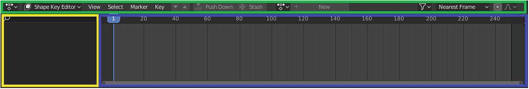
Dope Sheet ➤ Shape Key Editor
Yeah. It has the same setup as the Action Editor with a different purpose because it is specifically for editing shape keys.
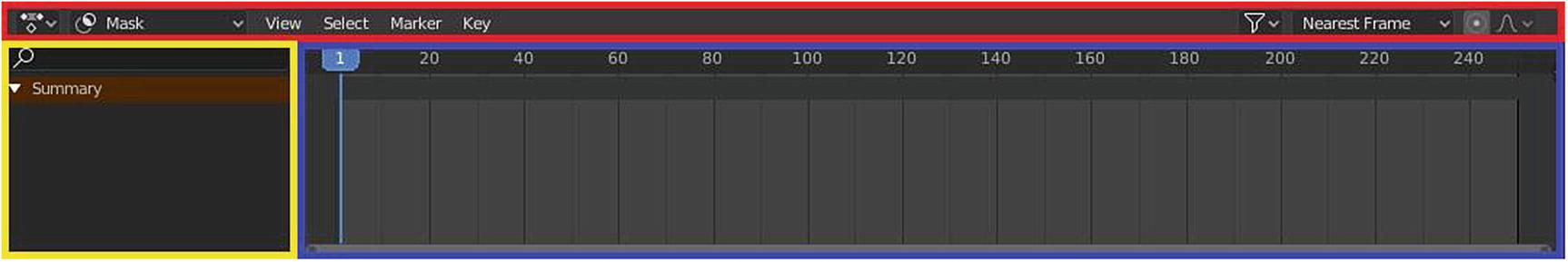
Dope Sheet ➤ Mask mode
As you can see, there is nothing much here aside from the Summary and Name filter in the Channel region, the View menu, Select menu, Marker menu, Key menu, Filters, Snapping and Proportional Editing Falloff for the Header region because it is specifically for editing mask data-blocks. Mask is a grayscale image that included or excluded parts of an image. A matte is applied as an alpha channel or it is used as a mix factor when applying color blend modes.
Masks can be created in the UV/Image and Movie Clip Editors, by changing the mode to Mask in the header. Masks have many purposes. They can be used in a motion tracking workflow to mask out, or influence a particular object in the footage. They can be used for manual rotoscoping to pull a particular object out of the footage, or as a rough matte for green-screen keying. Masks are independent from a particular image of movie clip, and so they can just as well be used for creating motion graphics or other effects in the compositor. Mask data-blocks contain multiple mask layers and splines. They are the most high-level entities used for masking purposes. Masks can be reused in different places, and hold global parameters for all entities they consist of.
Let’s proceed to the Cache File mode. This mode edits timings for Cache File data-blocks.
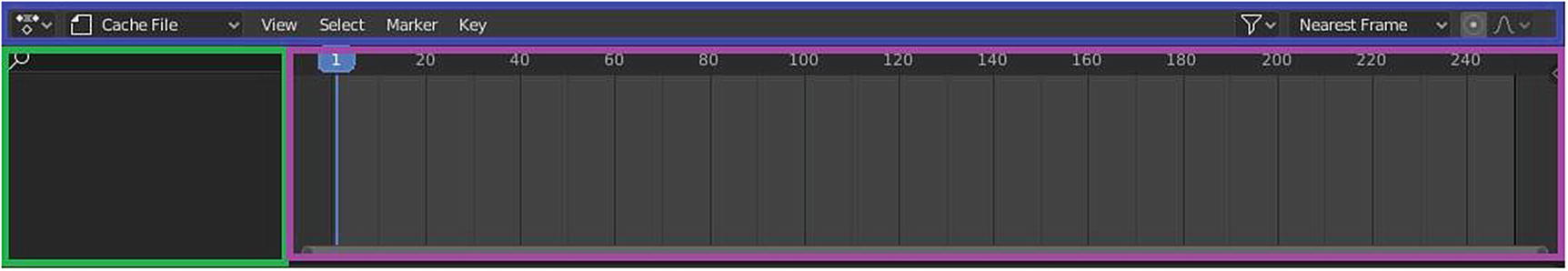
Dope Sheet ➤ Cache File mode
Cache File mode looks like the Dope Sheet mode. It only differs on its use. This is a new mode developed by the team. This Cache File mode is for working with Alembic files.
What is Alembic? Alembic is an open computer graphics interchange framework. Alembic distills complex, animated scenes into a non-procedural, application-independent set of baked geometric results. This distillation of scenes into baked geometry is exactly analogous to the distillation of lighting and rendering scenes into rendered image data.
Alembic is focused on efficiently storing the computed results of complex procedural geometric constructions. It is very specifically not concerned with storing the complex dependency graph procedural tools to create the computed results.
To simplify it, Cache File mode edits the Blender cache file. It is quite technical. The simplest way I can tell about this is it is a temporary file stored in your computer for your file as a backup.
Dope Sheet ➤ Grease Pencil Mode
Grease Pencil allows you to adjust the timing of the grease pencil tool’s animated sketches. It is especially useful for animators blocking out shots, where the ability to re-time blocking is one of the main purpose of the whole exercise.
Dope Editor ➤ Grease Pencil mode
The Channel region of this mode has Summary and the Name filter. The Header region has the View menu, Select menu, Marker menu, Channel menu, and Frame menu.
The Active Only button only shows Grease Pencil data-blocks used as part of the active scene.
The Channel region of the Grease Pencil shows the data-blocks containing the layers. Multiple blocks are used for each area. This channel contains the keyframes to which the layer binds.
It is also possible to copy sketches from a layer to other layers using the Copy and Paste buttons. This works in a similar way as copy/paste tools for keyframes in the Action Editor.
Sketches can also be copied from data-block to another using these tools. It is important to keep in mind that keyframes will only be pasted into selected layers, so layers need to be created for the destination areas too.
Insert Keyframe can be used for creating blank Grease Pencil frames at a particular frame. It will create blank frames if Additive Drawing is disabled; otherwise, it makes a copy of the active frame on that layer, and use that.
Grease Pencil Mode Header Menus
Grease Pencil mode’s Header menus
In Figure 5-15, only View and Marker menu remains the same. There are changes in Select menu, Channel menu and Frame menu.
Let’s discuss the three channels, starting with the Select menu.
After Current Frame (]) selects the keyframe after the current frame. Before Current Frame ([) selects the keyframe before the current frame. Between Selected Markers (Alt+K) selects all keyframes between selected markers. Columns on Selected Markers (Shift+K) selects all keyframes on selected markers. Column on Current Frame (Ctrl+K) selects all keyframes on current frame. Columns on Selected Keys (K) selects all keyframes on selected keys. Circle Select (C) selects keyframes using circle select. Border Axis Range (Alt+B) selects all keyframes within the specific region. Box Select (B) selects keyframes using box select. Invert (Ctrl+I) selects keyframes using inverse selection. None (Alt+A) deselects all currently selected keyframes. All (A) selects all keyframes.
What differs with this Select menu is that it doesn’t have Select Linked, Select Less, and Select More.
Let’s proceed to the Channel menu. Delete Channels (X) deletes all selection animation channels. Toggle Channel Setting (Shift+W) toggles specified setting on all selected animation channels. There are two options that appear after you click the command: Protect and Mute. Enable Channel Setting (Shift+Ctrl+W) enables specified setting on all selected animation channels. There are two options that appear after you click the command: Protect and Mute. Disable Channel Setting (Alt+W) disables specified setting on all selected animation channels. There are two options that appear after you click the command: Protect and Mute. Toggle Channel Editability (Tab) toggles editability of selected channels.
What differs between this channel menu to the previous ones are this doesn’t have Revive Disabled F-Curve, Move, Collapse Channels, Expand Channels, Extrapolation mode, Ungroup Channel, and Group Channel.
Transform transforms selected items. There are four options: Move (G), Extend (E), Slide (Shift+T), and Scale (S). Move moves selected items. Extend extends selected items. Slide slides selected items. Scale scales or resize selected items.
Snap snaps selected keyframes to the times specified. There are four options. Current Frame snaps selected keyframes to the current frame. Nearest Frame snaps selected keyframes to the nearest frame. Nearest Second snaps selected keyframes to the nearest second. Nearest Marker snaps selected keyframes to the nearest marker.
Mirror (Ctrl+M) flips selected keyframes over the selected mirror line. There are three options. By Times over Current Frame flips times of selected keyframes using the current frame as the mirror line. By Values over Value = 0 flips the values of selected keyframes example negative turn to positive or vice versa. By Times over First Selected Marker flips the time of selected keyframes using the first selected marker as the reference point.
Duplicate Keyframes makes a copy of all selected keyframes. Delete Keyframes remove all selected keyframes. Set Keyframe Type (R) sets type of keyframes for the selected keyframes by clicking the command and the option will pop up.
Timeline
Timeline is located at the bottom of the Animation workspace. Timeline gives the user a broad overview of a scene’s animation, by showing the current frame, the keyframes of the active object, the start and end frames of your animation sequence, as well as markers set by the user.

The look of Timeline in Animation workspace
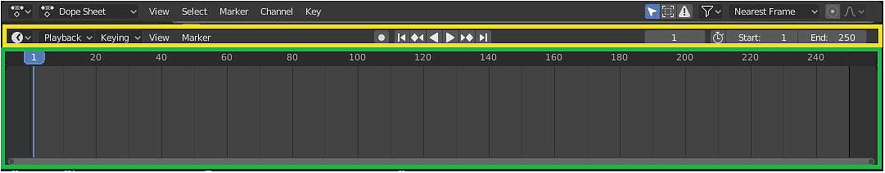
Timeline Editor at its full setup
You can only see the Dope Sheet Header region because the Timeline occupies the space of the Channel region and Main region of the Dope Sheet as we resize it. This is not specific for timeline. This is applied to all editors when you drag or resize an editor and extend it to the side of the other editor.
So let’s go back to the timeline. Figure 5-17 shows the default Timeline setup. By default, the Channel region is hidden, but you can make it appear by placing you mouse cursor on the small arrow next to the timeline; when your cursor turns to a double-sided arrow, drag it to the right.
Below the Header region is the Timeline region, where you see the animation flow. In the Header region, there are Playback, Keying, View, and Marker menus and Transport controls.
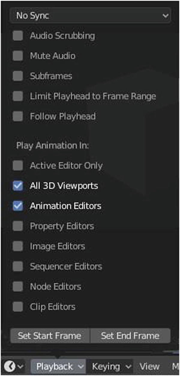
The Playback pop-over menu contains options for controlling animation playback. Sync mode synchronizes the playback if the scene is detailed and playback is slower than the set frame rate. This is shown in the 3D Viewport when you play the animation. There are three options. No Sync means no synchronization happens. Frame Dropping means drops frames when the playback is too slow. AV-Sync or Audio/Video Synchronization means to sync audio clock and drops frames when playback is slow.
Audio Scrubbing plays bits of the sound wave while you move the playhead with the left mouse button or keyboard arrow keys if your animation has sound. Mute Audio mutes sound from any audio source. Subframes displays and allows changing the current scene sub-frame. Limit Playhead to Frame Range doesn’t allow selecting frames outside of the playback range using the mouse. Follow Playhead follows current frame in the editors. Active Editor Only updates the Timeline while playing if the Animation Editors and All 3D Viewports are disabled. All 3D Viewports updates the 3D Viewport and the timeline while playing. Animation Editors updates the Timeline, Dope Sheet, Graph Editor, and Video Sequencer. Property Editors updates the property values in the UI while the animation is playing. Image Editors is the Image Editor in Mask mode. Sequencer Editors updates the Video sequencer while the animation is playing. Node Editors updates the Node Properties while the animation is playing. Clip Editors updates the Movie Clip Editor. Set Start Frame a button where you can use to choose where part of the timeline region you want to set your Start Frame. Set End Frame button allows you to choose where in the timeline region you want to set your end frame.
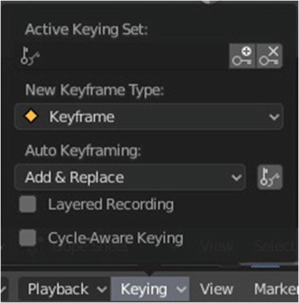
Keying Pop-over menu
The Keying pop-over menu contains options that affect keyframe insertion. With Active Keying Set, the keying sets are a set of keyframe channels in one. They are made so the user can record multiple properties at the same time. With a keying set selected, when you insert a keyframe, Blender will add keyframes for the properties in the active Keying Set. There are two small buttons with keys in its icons. Insert Keyframes inserts keyframes on the current frame for the properties in the active set. Delete Keyframes deletes keyframes on the current frame for the properties in the active set.
New Keyframe Type inserts keyframe types. There are five options. Keyframe is a normal keyframe. Breakdown is the breakdown state that mostly for transitions between key poses. Moving Hold is a keyframe that adds a small amount of motion around a holding pose. Extreme is an extreme state. Jitter is a filler and baked keyframe for keying on ones. Auto-Keyframing mode controls how the auto keyframe mode works.
There are two options. Add & Replace adds or replaces existing keyframes. Replace replaces existing keyframes. Auto Keying Set the one with two keys icon. Auto Keyframe inserts new keyframes for the properties in the active Keying Set. Layered Recording adds a new NLA Track and strip for every loop/pass made over the animation to allow non-destructive tweaking. Cycle-Aware Keying applies special handling to preserve the cycle integrity when inserting keyframes into trivially cyclic curves.
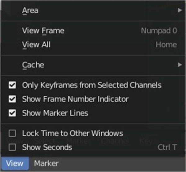
Timeline ➤ View menu
Let’s discuss the View menu. Area allows you to choose how the editor is displayed. There are five options: Horizontal Split, Vertical Split, Duplicate Area into New Window, Toggle Maximize Area (Ctrl+spacebar), and Toggle Fullscreen Area (Ctrl+Alt+spacebar). View Frame (Numpad 0) resets viewable area to show range around current frame. View All (Home) resets viewable area to show full keyframe range. Cache gives you an option to show caches. There are seven options: Show Cache, Softbody, Particles, Cloth, Smoke, Dynamic Paint, and Rigid Body.
What is a cache? It is a block of memory for temporary storage of data likely to be used again. It is made up of a pool of entries. Each entry has associated data, which is a copy of the same data in some backing store. To put it simply, it is data that is saved to be used again. This is how Cache works; it makes your usual tasks easy.
OK, let’s go back to the View menu. Only Keyframes from Selected Channels considers keyframes for active Object and/or its selected bones only. Show Frame Number Indicator shows the frame number beside the current frame indicate line. Show Marker Lines shows a vertical line for every marker. Lock Time to Other Windows synchronizes the horizontal panning and scale of the current editor with the other editors and this way you always have these editors (Graph Editor, Dope Sheet, NLA) showing an identical part of time you work on. Show Seconds (Ctrl+T) shows the time in the x axis and the playhead as frames or as seconds.
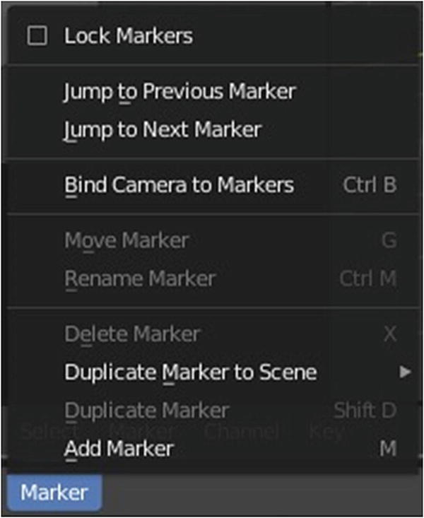
Timeline ➤ Marker menu
As you can see in the Marker menu, there are commands that are disabled. It’s because there are no markers in the Timeline. Most of the Marker’s command will only work when your cursor are in the marker itself or when you hover your cursor to the marker, even when using shortcut keys.
Lock Markers prevents marker editing. Jump to Previous Marker jumps to previous marker from the current marker selected. Jump to Next Marker jumps to next marker from the current marker selected. Bind Camera to Markers (Ctrl+B) binds the selected camera to a marker on a current frame; and in this way, the operator allows markers to set the active object as the active camera. Move Marker (G) moves selected time marker. Rename Marker (Ctrl+M) renames first selected marker. Delete Marker (X) deletes selected time marker. Duplicate Marker to Scene copies selected marker to another scene. Duplicate Marker (Shift+D) duplicates selected marker. Add Marker adds a new time marker.
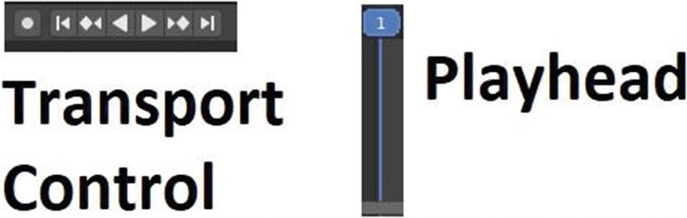
Transport Control and Playhead
These buttons and transport controls set, play, and rewind the playhead. The playhead is the blue vertical line (see Figure 5-22); the current frame number is at the top.
Let’s discuss the Transport controls. Auto Keyframe adds and/or replaces existing keyframes for the active object when you transform it in the 3D Viewport. Jump to start sets the cursor to the start of frame range. Jump to Previous Keyframe sets the cursor to the previous keyframe. Rewind plays the animation sequence in reverse. When playing the play buttons switch to a pause button. Play plays the animation sequence. Again when playing the play buttons switch to a pause button. Jump to Next Keyframe sets the cursor to the next keyframe. Jump to End sets the cursor to the end of frame range. Pause stops the animation.

Frame Controls
Current Frame is the first rectangle; it shows the current frame and the position of the playhead. Preview Range is the clock icon; it is a temporary frame range used for previewing a smaller part of the full range. The preview range only affects the viewport not the rendered output. Start Frame shows the starts frame of the animation or playback range. End Frame shows the end frame of the animation or playback range.
Graph Editor
The Graph Editor allows users to adjust animation curves over time for any animatable property. It also has three main parts: Main region, Header and Sidebar region, like Dope Sheet Editor and Timeline. Let’s discuss its basic settings or common settings.

Graph Editor (Header region, yellow; Channel region, green; Main region, light blue)
In Figure 5-24, the sidebar is hidden by default. You can bring it up by pressing N in your keyboard.
The Normalize button normalizes curves so the maximum or minimum point equals 1.0 or –1.0.
Only Selected (the arrow icon) only includes curves related to the selected objects and data.
Display Hidden (the dashed small box icon) includes curves from bones/objects that aren’t visible.
Show Errors (the warning triangle icon) only includes curves and drivers that are disabled or have errors. You can select the three at once.
Create Ghost Curves creates snapshot of selected F-curves as background aid for active Graph Editor.
Filters (the funnel icon) a pop-over menu where you can set what data-block to show in the Graph Editor. The Filters are the same as Dope Sheet mode.
Pivot Point where you set the pivot point for the rotation. There are three options: Bounding Box Center, 2D cursor, and Individual Center.
Bounding Box Center is the center of the selected keyframes.
2D cursor is the center of the 2D cursor. It is Playhead+the cursor.
Individual Centers rotates the selected keyframe Bezier handles.
In the Graph Editor, there is a Snapping tool. There are six options: No Auto snap, Frame Step, Second Step, Nearest Frame, Nearest Second, and Nearest Marker.
No Auto Snap means no snapping at all. Frame Step means snap to 1.0 frame intervals. Second Step means snap to one-second intervals. Nearest Frame means snap to actual frames. Nearest Second means snap to actual seconds. Nearest Marker means snap to nearest marker. By default, it is set to Nearest Frame.
Proportional Editing Falloff has eight options: Random, Constant, Linear, Sharp, Inverse Square, Root, Sphere, and Smooth.
Header menus for Graph Editor
View Menu
The View menu of the Graph Editor have that the View menu of Dope Sheet doesn’t have. Only Selected Keyframes Handles only shows and edit handles of selected keyframes. Only Selected Curve Keyframes only keyframes of selected F-curves are visible and editable. Show Handles (Ctrl+H) shows the handles of Bezier control points. Use High Quality Display displays F-curve using anti-aliasing and other fancy effects. Shows 2D cursor command shows a 2d cursor. When you used it, you will notice a change in the line of the Graph Editor.
Dope Sheet has Show Curve Extreme, Show Handles, and Interpolation and Multi-word Match Search that the Graph Editor’s View menu doesn’t have.
In Figure 5-25, most of the commands, especially in Select menu, are disabled. This is because there is nothing in the Graph Editor to work on.
Select Menu
The only difference between the Graph Editor’s and Dope Sheet’s Select menu is Border Include Handles. It selects all keyframes within the specified region.
Marker Menu
For Marker menu, the only difference between Graph Editor and Dope Sheet is that the Sync Marker isn’t available in Graph Editor Marker menu. I’d like to note again that Markers denote frames with key points or significant events within an animation.
Channel Menu
We can see that the Graph Editor’s Channel menu have Collapse Channel, Expand Channel, Reveal Curves, Hide Unselected Curves, Hide Selected Curves. Dope Sheet’s Channel menu doesn’t have them, but all of what you can see in its menu is carried.
I’d like to remind you that Extrapolation defines the behavior of a curve before the first and after the last keyframes while Interpolation mode is a mode for interpolation, or process calculating new data between points known as value, between the current and next playframe.
Key Menu
The difference between the Key menu of Graph Editor and the Dope Sheet are the Discontinuity Euler Filter, Bake Curve, Smooth Keys, Easing Type, Bake Sound to F-curves and Add F-curves Modifiers of Graph Editor and Key Frame type of the Dope Sheet.
Sample Project
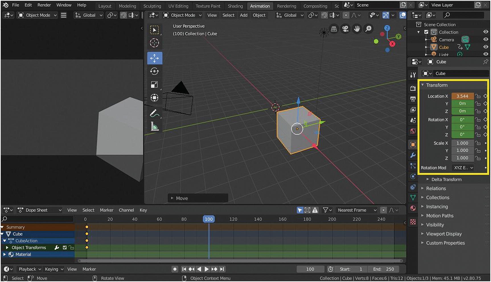
As usual, this is a step-by-step procedure. Let’s do a simple animation, first, with the default cube. Figure 5-26 to Figure 5-39 shows the step-by-step procedure.
First Step

Second step
The view in Timeline

Third Step
Moving on the Frame
Moving the Object

Fourth Step
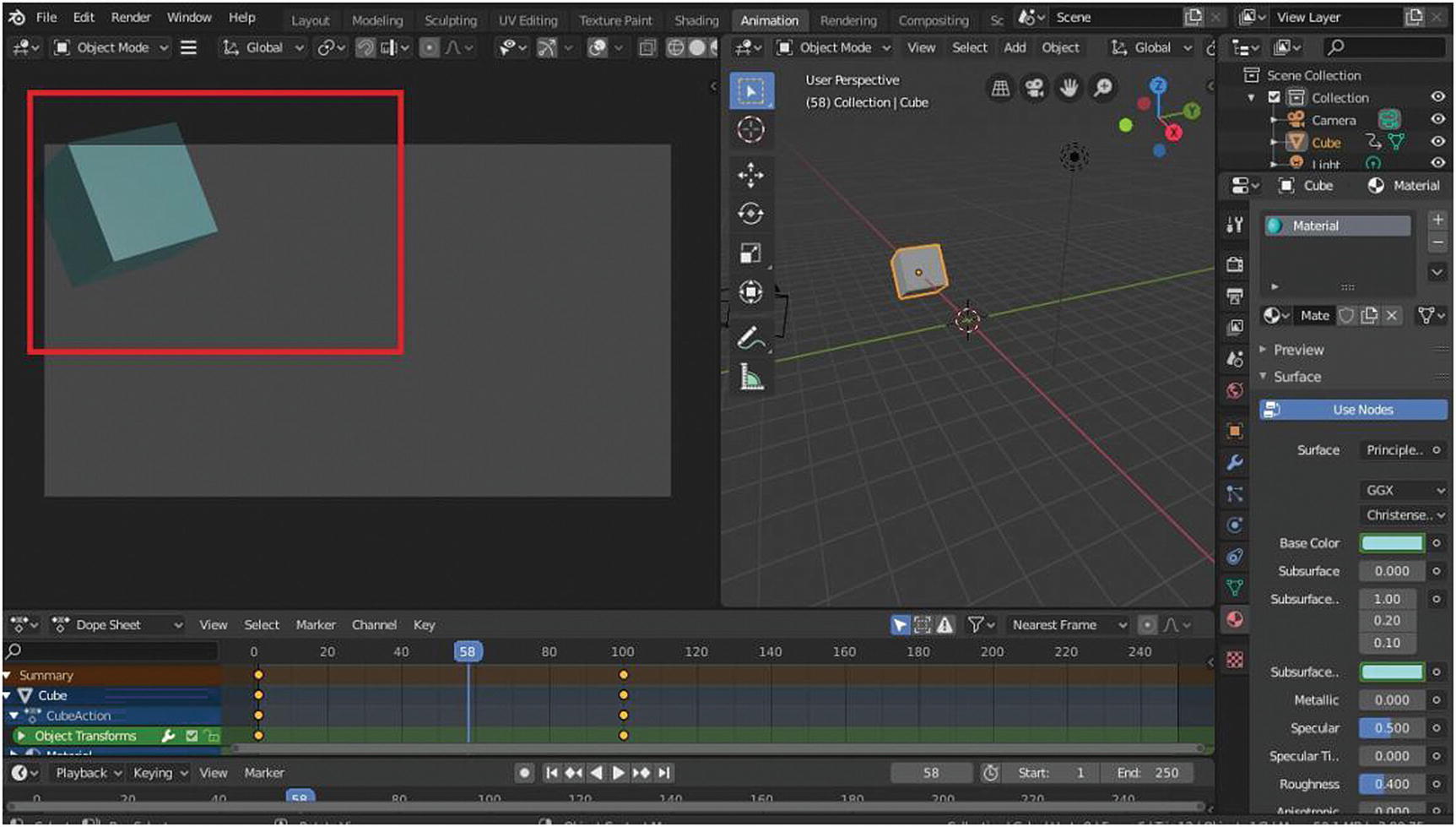
Rendered view in 3D

Rendered with 3D Viewport
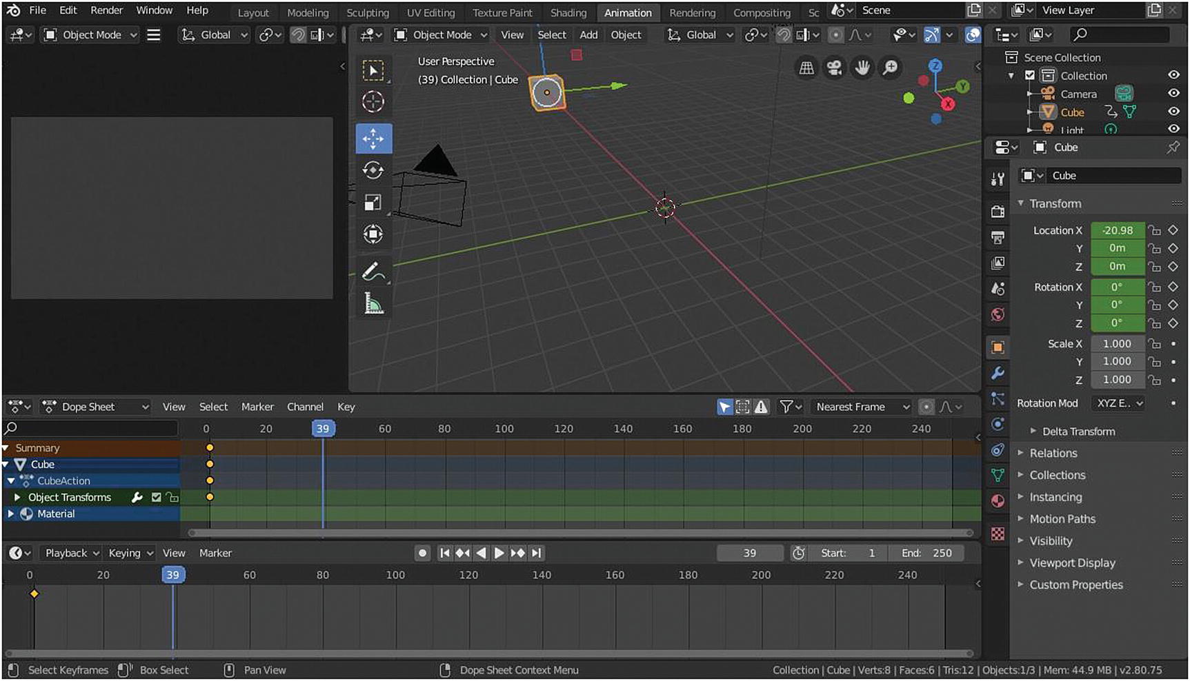
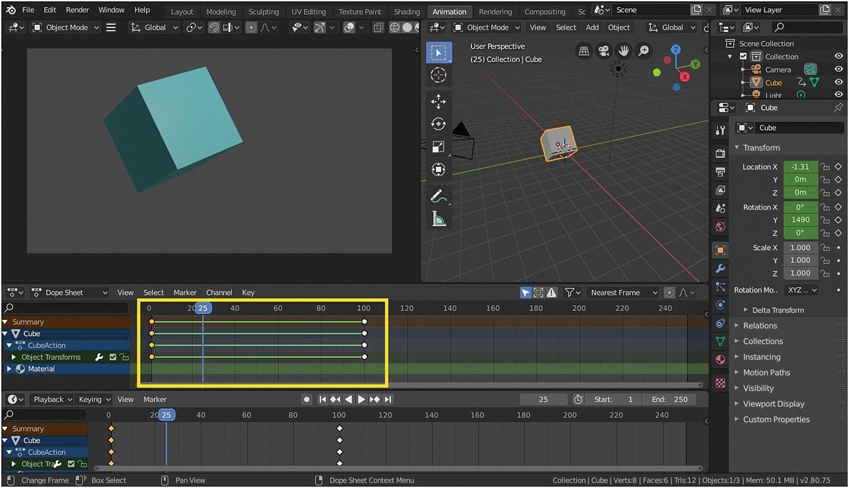
Observe the changes happened in the cube by looking at Figure 5-34.
As you can see, when we don’t have keyframes in between, the animation continues. When the playhead is in between, the color of the Location value, Rotation value, Base color value, and Subsurface value is in green, which represents animation from the first keyframe to the second keyframe.
Interpolation mode
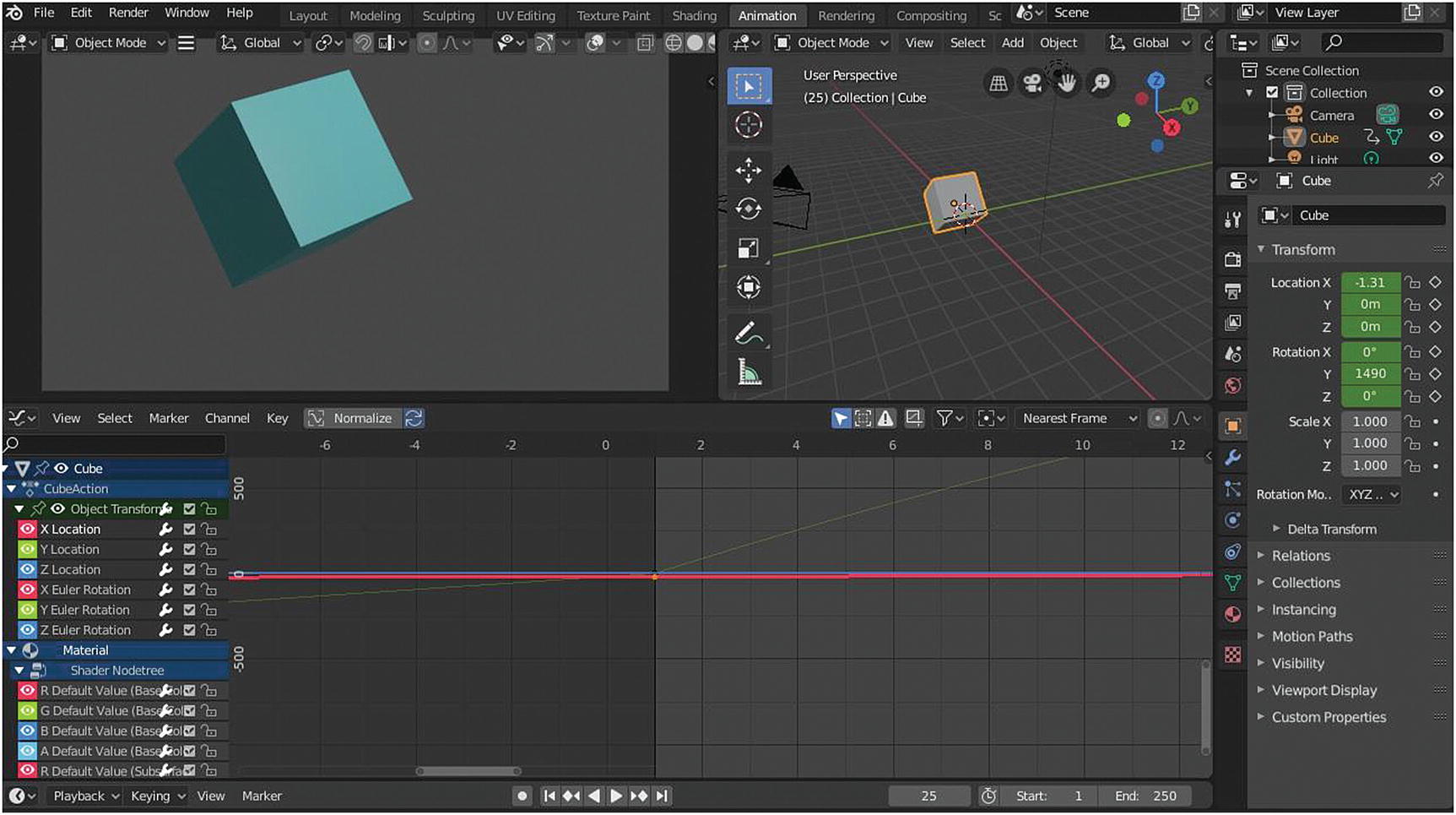
Graph Editor
Figure 5-37 shows how it looks in the Action Editor. As you can see, it shows simple data. It doesn’t show anything related to the materials.

Action Editor

Shape Key Editor, Grease Pencil and Mask
What is Shape Keys? Shape keys support different target shapes (such as facial expressions) to be controlled. This deforms objects into new shapes for animation. In other terminology, shape keys may be called morph targets or blend shapes. This is helpful in character animation and the likes.
Mask mode doesn’t have any data in it because we don’t have anything that is in mask. Grease Pencil mode creates 2D animation.
Rendering Workspace
Rendering is the process of turning a 3D scene into a 2D image. As you know, Blender includes three render Engines with different strengths. Eevee is a physically based real-time renderer. Cycles is a physically based path tracer. Workbench is designed for layout, modeling, and previews.
What the render looks like is defined by cameras, lights, and materials. These are shared between Eevee and Cycles; however, some features are only supported in one or the other.
Renders can be split up into layers and passes, which can then be composited together for creative control or to combine layers with real footage. Freestyle can add non-photorealistic line rendering.
Blender supports interactive 3D Viewport rendering for all render engines, for quick integration of lighting and shading. Once this is done, the final quality image or animation can be rendered and output to disk.
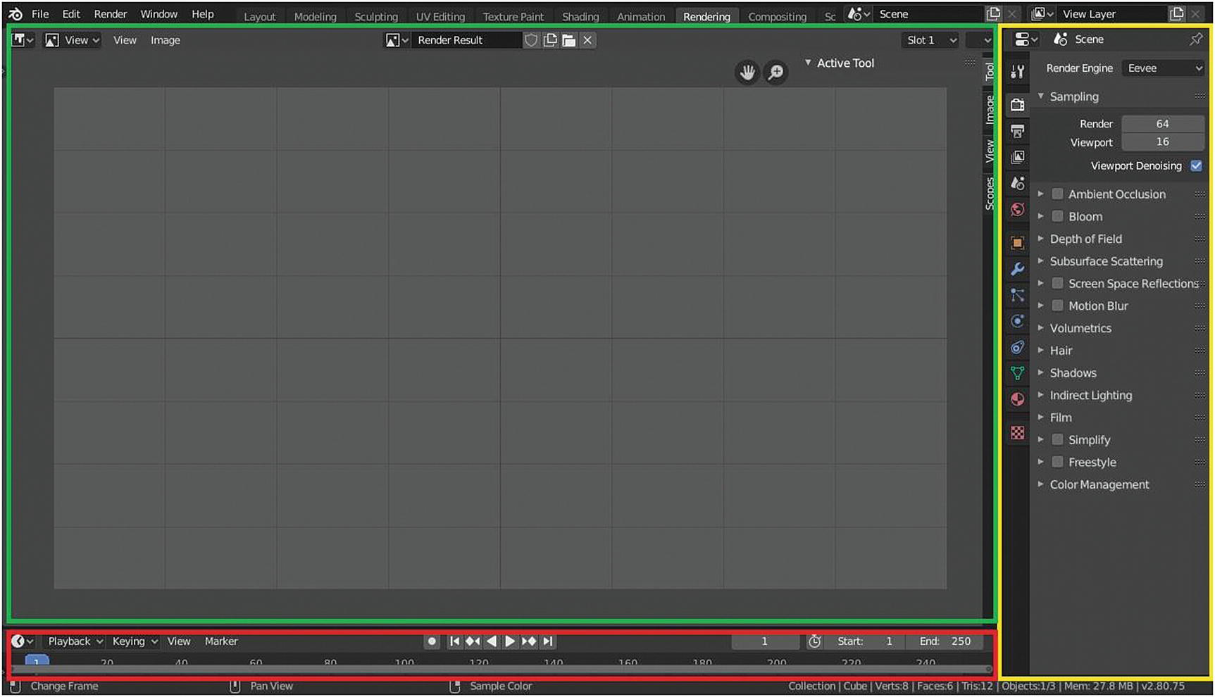
Rendering workspace. (Image Editor: green; Properties: yellow; and Timeline: red)
The Image Editor differs from the Image Editor in the Shading workspace. Let’s discuss the Image Editor in the Rendering workspace.
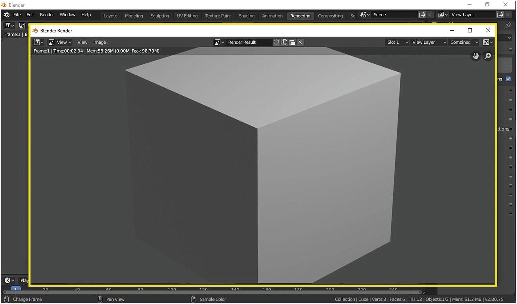
Rendered image
As you can see in Figure 5-40, when you rendered an image/animation, another window is being opened and behind it is the main window of Blender.

Rendered image in the Rendering workspace
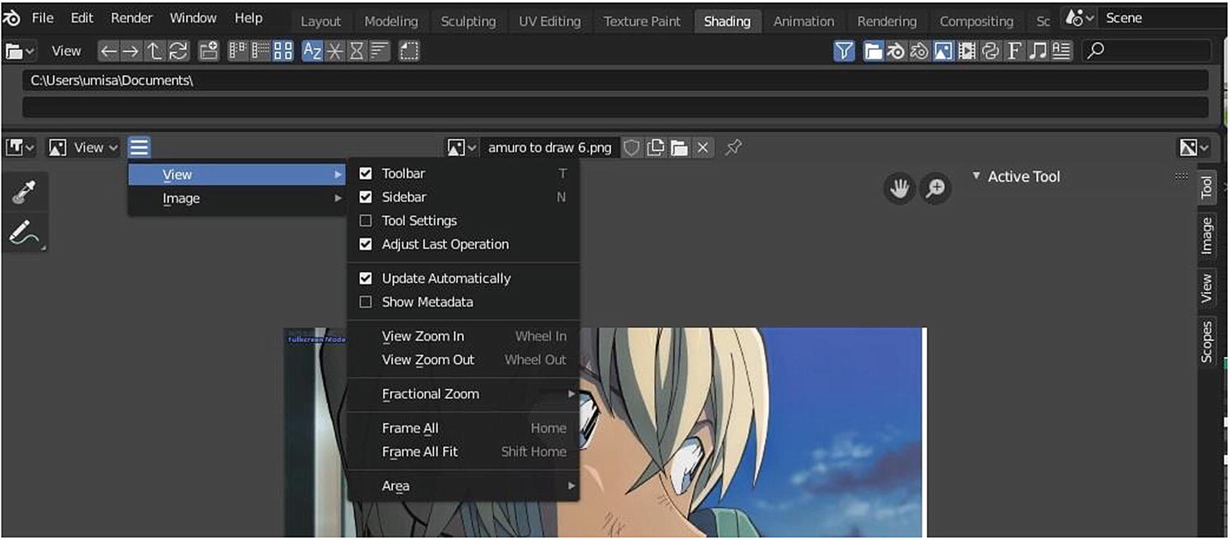
Image Editor in the Shading workspace
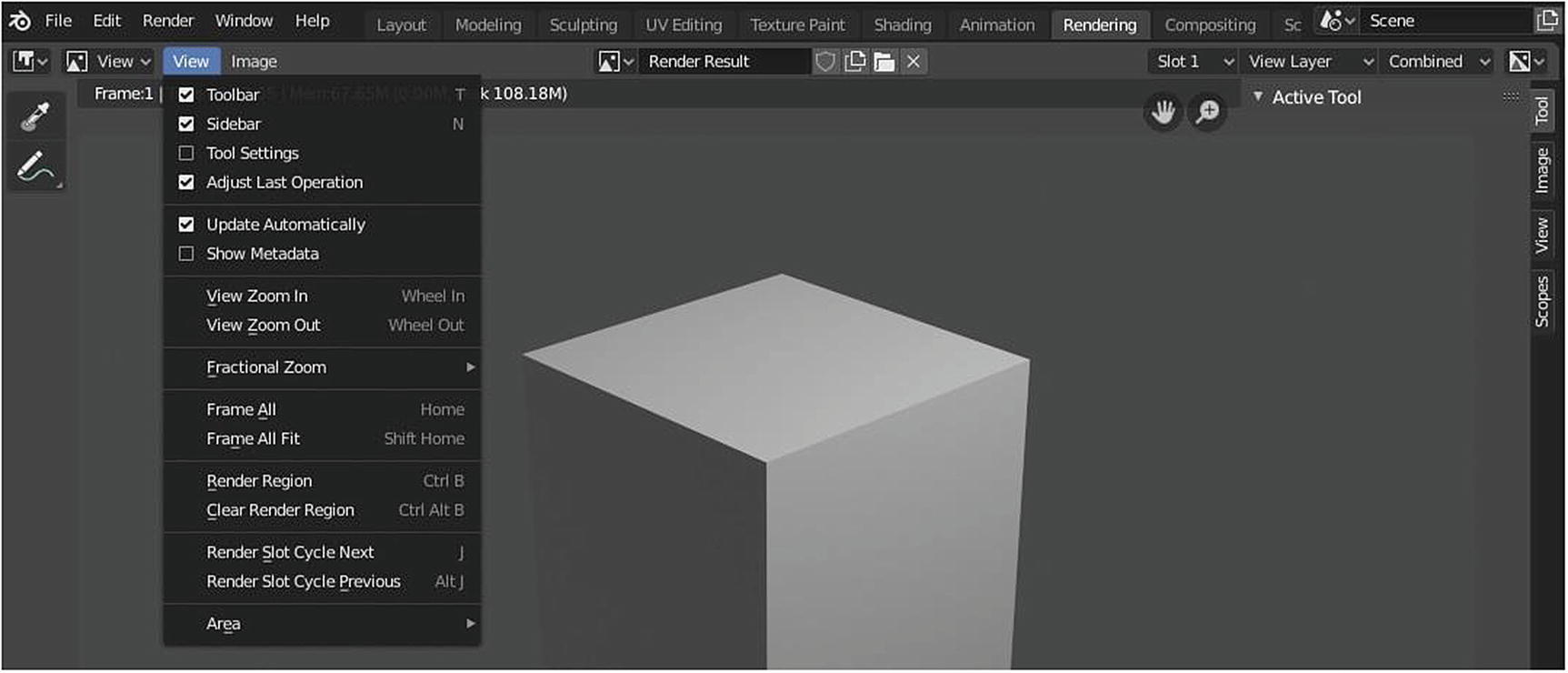
Image Editor in Rendering workspace
They both have the same tools in the toolbar: Sample and Annotate tools. They both have the three modes View, Paint, and Mask. In the Image Editor of rendering workspace, there is the Fake User button, New Image button, Open button, and Delete button; but it doesn’t have the Image Pin button. They both have Tool, Image, View, and Scope panels. But as in the View menu, there are differences. There are commands in the Rendering workspace’s Image Editor that isn’t available in the Image Editor.
Header Menus

View menu and Image menu of Image Editor in Rendering workspace
Again, the View menu is pretty self-explanatory.
The two interesting options from the Image menu are: Open Cached Render (Ctrl+R) reads all the current scene’s view layers from cache as needed. Edit Externally edits image in an eternal application.

Tool, Image, View and Scope panel
These panels are almost the same as the Shading workspace’s Image Editor. What is different are Source, Color Space, Alpha, Image Path, a checkbox for View as Render and metadata. Here you see render slots.

Slot select menu
If you didn’t change your slot here, click the render image; whatever rendered image was placed in the slot is replaced by the new rendered image.
Sample Project

Workbench Rendered result
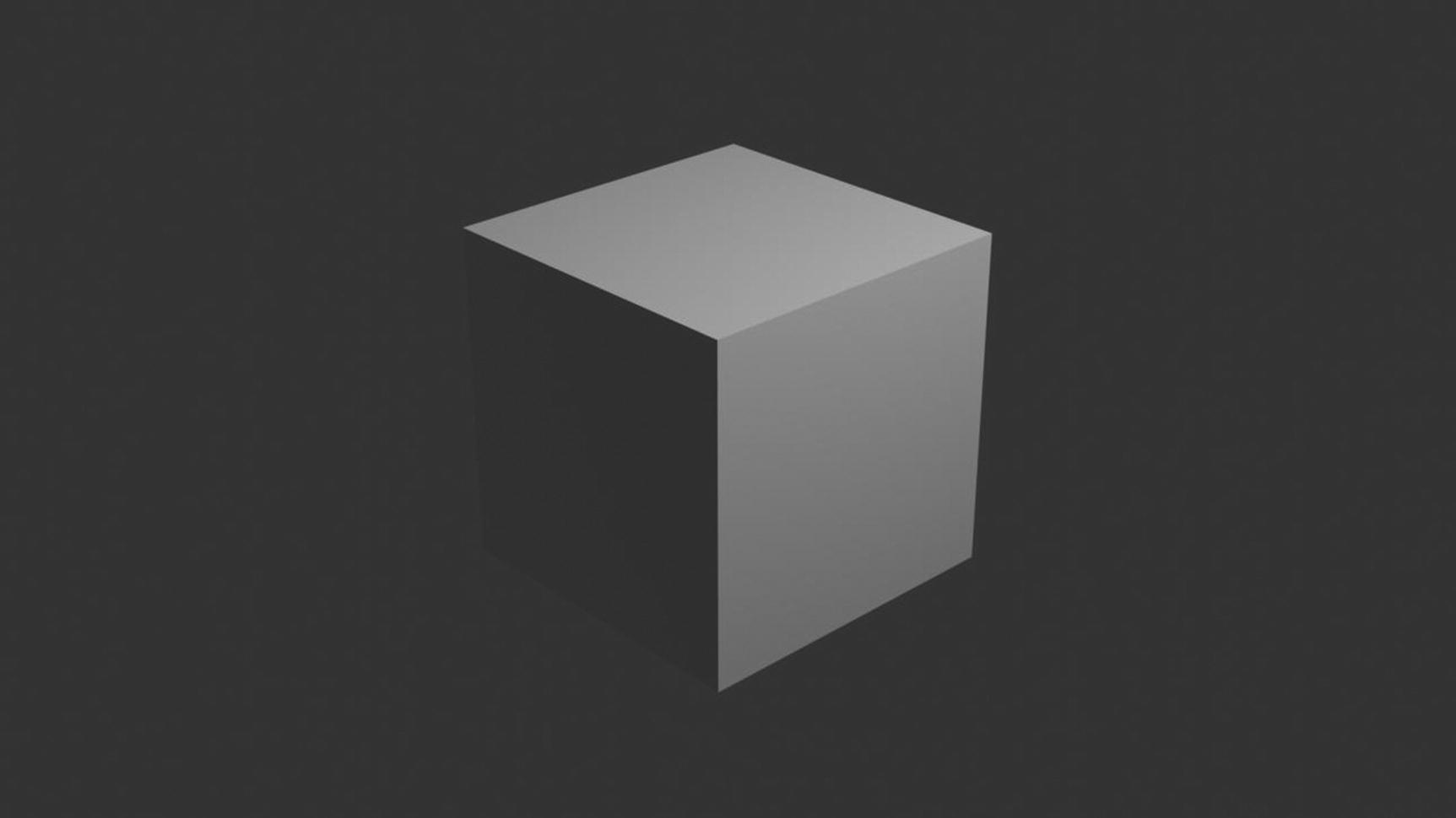
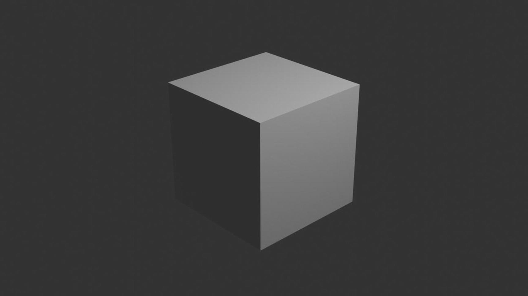
Workbench’s differences can easily be noticed with this default cube because of its lighting. Eevee and Cycles differ but they are hard to distinguish because at first glance of this simple project, they are similar. Actually, Cycles is more detailed than Eevee and the shadows in Cycles are darker if you look at it closely.
A complex project can make you learn differences: character modeling uses hair particles, architectural visualization uses different kinds of lighting, and so forth.
Camera Fundamentals
The camera is one of the most important parts in rendering a scene.
Capturing an ideal shot isn’t that simple. There are a lot of things to consider but I’ll give you some of the basic things so that you can apply when rendering an image.
First is the Aperture. This refers to the diameter of the hole inside the lens. A change in aperture alters the size of this hole, allowing more or less light into the camera, which also has an effect on the depth of field of your final image. You can image this as something like a pupil of your eye. The wider the aperture, the more light is allowed in.
Second, there is the Shutter Speed. The mirror flips up and the shutter opens, recording the light present onto the sensor. The speed at which this happens determines the exposure length as well as the amount of motion blur. After the light passes the aperture, it then reaches the shutter.
Third, there is the ISO. The sensor captures the light and is controlled by the ISO. The higher you set, the more sensitive it is, but it’ll also capture more digital noise. Once the light passes the Aperture and been filtered by the shutter speed, it reaches the sensor. This is where the ISO comes in. As you turn the ISO number up, you increase the exposure but at the same time, the quality of the image decreases.
I’ll stop with these basic camera fundamentals. You can learn more at http://expertphotography.com.
I left out three things in the Properties section in Chapter 2: Objects Constraints, Particles, and Physics. Let’s talk about them now.
Note
There’s no sample project for Object Constraints, Particles and Physics because I don’t think it is easy to demonstrate it with figures so our discussion for these three is a thorough tour to give you an idea what’s available in Blender. The rest is up to your imagination.
Object Constraints
Constraints are a way to control an object’s properties, for example its location, rotation or scale, using either plain static value or another object called target.

Object Constraints
You can control an object’s animation through the targets used by its constraints. Indeed, these targets can then control the constraint’s owner’s properties, and hence, animating the targets will indirectly animate the owner.
You can animate constraints’ settings.
Constraints in Blender work with Objects and Bones. Constraints work in combination with each other to form a Constraint Stack.
Constraints are a fantastic way to add sophistication and complexity to a rig but be careful not to rush in too quickly, piling up constraints until you lose all sense of how they interact with each other.
Constraints are divided into four categories: Motion Tracking, Transform, Tracking, and Relationship.
Motion Tracking Constraints
Let’s discuss the constraints under Motion Tracking: Camera Solver, Follow Track, and Object Solver.
Camera Solver Constraint gives the owner (object) of the constraints the location and rotation of the solved camera motion. The solved camera motion is where the Blender reconstructs the position of the physical, real-world camera, when it filmed the video footage, relative to the thing being tracked. This constraints only works after you have set up a minimum of eight markers and clicked Solved Camera Motion in Movie Clip Editor ➤ Toolbar ➤ Solve ➤ Solve Camera Motion.

Camera Solver Constraint settings
Active Clip makes the constraints receive tracking data from the Movie Clip Editor but an option appears to choose from other clips. Constraints to F-Curve applies the constraint creating Keyframes for the transform. Influence is the amount of constraint on the final solution.
Follow Track Constraint makes objects have the same position at a frame as the track has and the motion of this object happens on a single plane defined by the camera and the original position of the object.

Follow Track Constraint
Active Clip makes the constraints receive tracking data from the Movie Clip Editor but an option appears to choose from other clips. 3D position uses the 3D position of the track to the parent. Undistort parents to the undistorted position of the 2D track. Frame Method defines how the footage is fitted in the camera frame. Camera selects the camera to which the motion is parented to, and if active, an empty scene camera is used. Depth Object constraint objects are projected onto the surface of this depth object, which can create facial makeup visual effects when this field is set. Constraint to F-curve creates F-curve for the objects that copies the movement cause by the constraints. Influence is the amount of constraint on the final solution.
Object Solver Constraint gives the owner of this constraint, the location, and rotation of the Solved Object Motion.
Note
Don’t be confused, okay? Camera Solver Constraint is for Solved Camera Motion. Object Solver Constraint is of Solved Object Motion. Camera ➤ Camera, Object ➤ Object.
The Solved Object Motion is where Blender thinks the physical, real-world (tracked) object was, relative to the camera that filmed it. This constraint only works after you have set up a minimum of eight markers and clicked Solved Object Motion in Movie Clip Editor ➤ Toolbar ➤ Solve ➤ Solve Camera Motion or Movie Clip Editor ➤ Sidebar region ➤ Objects.
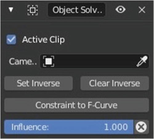
Object Solver Constraint
Active Clip makes the constraints receive tracking data from the Movie Clip Editor but an option appears to choose from other clips. Object selects a tracked object to receive transform data from. Camera selects the camera to which the motion is parented to and if active empty scene camera is used. Set Inverse moves the origin of the object to the origin of the camera. Clear Inverse moves the origin of the object back to the spot set in the Movie Clip Editor. Constraints to F-curve applies the constraint creating keyframes for the transform. Influence is the amount of constraint on the final solution.
Transform Constraints
Let’s proceed to the constraints under Transform: Copy Location, Copy Rotation, Copy Scale, Copy Transforms, Limit Distance, Limit Location, Limit Rotation, Limit Scale, Maintain Volume, Transformation, and Transform Cache.
Copy Location Constraint forces its owner to have the same location as its target.

Copy Location Constraint
Target is the data ID selects the constraints target and is not functional (red state) when it is none. XYZ controls the axes that are constrained. Invert inverts their respective preceding coordinates. Offset allows the owner to be moved using its current transform properties relative to its target’s position. Space is the standard conversion between spaces. Influence is the amount of constraint on the final solution.

Copy Location Constraint
Copy Rotation Constraint forces its owner to match rotation of its target.
Figure 5-55 shows its settings.
Target is the data ID selects the constraints target and is not functional (red state) when it is none. XYZ controls the axes that are constrained. Invert inverts their respective rotation values. Offset allows the owner to be rotated relative to its target’s orientation. Space is standards conversion between spaces. Influence is the amount of constraint on the final solution.
Copy Scale Constraint forces its owner to have the same scale as its target.

Copy Scale Constraint
Target is the data ID selects the constraints target and is not functional (red state) when it is none. XYZ controls along which axes the scale is constrained. Power allows raising the copied scale to the specified arbitrary power. Offset the constraints combines the copied scale with the owner’s scale instead of overwriting it. Additive uses addition instead of multiplication in the implementation of the Offset option. Space means standards conversion between spaces. Influence is the amount of constraint on the final solution.
Copy Transforms Constraint forces its owner to have the same transforms as its target.
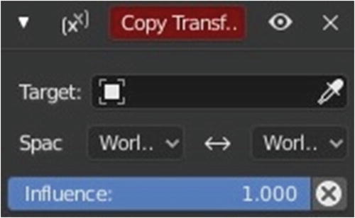
Copy Transforms Constraint
Target is the data ID selects the constraints target and is not functional (red state) when it is none. Space means standards conversion between spaces. Influence is the amount of constraint on the final solution.
Limit Distance Constraint forces its owner to stay either further from, nearer to, or exactly at a given distance from its target. In other words, the owner’s location is constrained outside, inside, or at the surface of a sphere centered on its target. When you specify a new target, the Distance value is automatically set to correspond to the distance between the owner and this target.
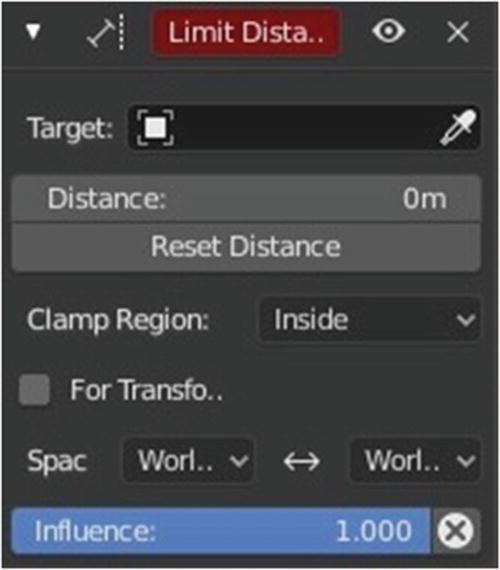
Limit Distance Constraint
Target is the data ID selects the constraints target and is not functional (red state) when it is none. Distance sets the limit distance. Reset Distance resets distance value when clicked so that it corresponds to the actual distance between the owner and its target. Clamp Region allows you to choose how to use sphere defined by the Distance setting and target’s origin. There are three options. Inside owner is constrained inside the sphere. Outside owner is constrained outside the owner. Surface owner is constrained on the surface of the sphere. For Transform restricts the resulting transform property values. Space means standards conversion between spaces. Influence is the amount of constraint on the final solution.
Limit Location Constraint restricts the amount of allowed translations along each axis, through lower and upper bounds.
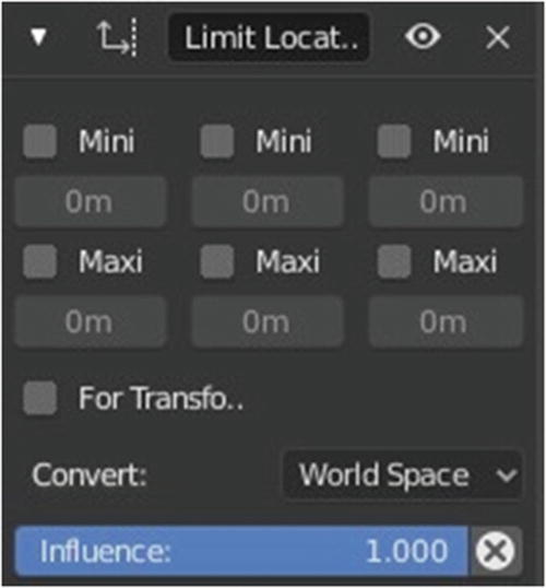
Limit Location Constraint
Mini XYZ enables the lower boundary for the location of the owner’s origin along the x, y, and z axes of the chosen space. The Mini XYZ number field controls the value of Minimum limit. Maxi XYZ enables the upper boundary for the location of the owner’s origin along respectively the X Y and Z axes of the chosen Space. The Maxi XYZ number field controls the value of Maximum limit. For Transform the owner’s transform properties are limited by the constraint because the owner can still have coordinates out of bounds. Convert allows you to choose in which space to evaluate its owner’s transform properties. Influence is the amount of constraint on the final solution.
Limit Rotation Constraint restricts the amount of allowed rotations around each axis, through lower and upper bounds.

Limit Rotation Constraint
Limit XYZ enables the rotation limit around respectively the X, Y and Z axes of the owner, in the chosen Space. Min/Max number fields control the value of their lower and upper boundaries. For Transform the owner’s transform properties are limited by the constraint because the owner can still have coordinates out of bounds. Convert allows you to choose in which space to evaluate its owner’s transform properties. Influence is the amount of constraint on the final solution.
Limit Scale Constraint restricts the amount of allowed scaling along each axis, through lower and upper bounds. This constraint does not tolerate negative scale values when you add it to an object or bone, even if no axis limit is enabled. With the For Transform button, as soon as you scale your object, all negative scale values are instantaneously inverted to positive ones and the boundary settings can only take strictly positive values.
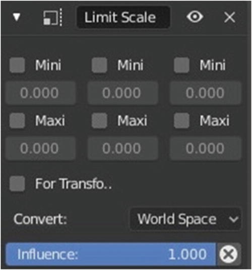
Limit Scale Constraint
Mini XYZ enables the lower boundary for the scale of the owner along, respectively, the X, Y and Z axes of the chosen Space. The Mini XYZ number field controls the value of Minimum limit. Maxi XYZ enables the upper boundary for the scale of the owner along, respectively, the X, Y and Z axes of the chosen Space. The Maxi XYZ number field controls the value of Maximum limit. With For Transform, the owner’s transform properties are limited by the constraint because the owner can still have coordinates that are out of bounds. Convert allows you to choose in which space to evaluate its owner’s transform properties. Influence is the amount of constraint on the final solution.
Maintain Volume Constraint limits the volume of a mesh or a bone to a given ratio of its original volume.

Maintain Volume Constraint
Mode specifies how the constraint handles scaling of the non-free axes. There are three options. Strict overrides non-free axis scaling to strictly maintain the specified volume. Uniform maintains the volume as specified only when the pre-constraint scaling is uniform. Single Axis maintains the volume only when the object is scaled on its free axis. Free free-scaling axis of the object. Volume sets the bone’s rest volume. Convert allows you to choose which space to evaluate its owner’s transform properties. Influence is the amount of constraint on the final solution.
Transformation Constraint is more complex and versatile than the other transform constraints. It allows you to map one type of transform properties of the target, to the same or another type of transform properties of the owner, within a given range of values. You can also switch between axes and use the range values not as limits, but rather as markers to define a mapping between input (target) and output (owner) values.

Transformation Constraint
Target is the data ID selects the constraints target and is not functional (red state) when it is none. Extrapolate’s min and max values bound the input and output values. all values outside these ranges are clipped to them. When you enable this button, the min and max values are no longer strict limits but rather markers defining a proportional (linear) mapping between input and corresponding output values. Source contains the input (from target) settings. Destination contains the output (to owner) settings. Space means standard conversion between spaces. Influence is the amount of constraint on the final solution.
Transform Cache Constraint streams animations made at the transformation matrix level.

Transform Cache Constraint
The Cache File data-block menu selects the Alembic file. File Path is the path to the Alembic file. Is Sequence (when file is opened) determines whether the cache file is separated in a series of files. Override Frame (when file is opened) is an option to use a custom frame for looking up data in the cache file instead of using the current scene frame. Manual Transform Scale (when file is opened) is the value by which to enlarge or shrink the object with respect to the world’s origin. Object Path (when file is opened) is the path to the Alembic object inside the archive. Vertices/Faces/UV/Color (when file is opened) determines the type of data to read for a mesh object, respectively. Influence is the amount of constraint on the final solution.
Tracking Constraints
Let’s proceed to the constraints under the Tracking category: Clamp To, Damped Track, Locked Track, Stretch To, and Track To.
Clamp To Constraint clamps an object to a curve. It is very similar to the Follow Path constraint, but instead of using the evaluation time of the target curve, Clamp To will get the actual location properties of its owner (those shown in the Transform panel), and judge where to put it by mapping this location along the target curve.

Clamp To Constraint
Target is the data ID to select the constraints target and is not functional (red state) when it is none. Main controls which global axis is the main direction of the path. Cyclic as soon as the object reaches one end of the curve it is instantaneously moved to its other end. Influence is the amount of constraint on the final solution.
Damped Track Constraint constrains one local axis of the owner to always point towards Target.
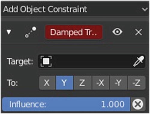
Damped Track Constraint
Target is the data ID selects the constraints target and is not functional (red state) when it is none. To is the axis of the object you want to point at the Target object. Influence is the amount of constraint on the final solution.
Locked Track Constraint is a Track To constraint, but with a locked axis. Hence, the owner can only track its target by rotating around this axis, and unless the target is in the plane perpendicular to the locked axis, and crossing the owner, this owner cannot really point at its target.

Locked Track Constraint
Target is the data ID selects the constraints target and is not functional (red state) when it is none. To is the tracking local axis. Lock is the locked local axis. Influence is the amount of constraint on the final solution.
Stretch To Constraint causes its owner to rotate and scale its y axis toward its target. So it has the same tracking behavior as the Track To constraint. However, it assumes that the y axis is the tracking and stretching axis, and does not give you the option of using a different one.

Stretch To Constraint
Target is the data ID selects the constraints target and is not functional (red state) when it is none. Rest Length sets the rest distance between the owner and its target. Reset recalculates the Rest Length value so that it corresponds to the actual distance between the owner and its target. Volume Variation controls the amount of volume variation exponentially to the stretching amount. Volume Min/Volume Max limits for the volume preservation to a minimum and maximum scaling each by a Bulge factor. Smooth is the smoothness factor to make limits less visible. Volume controls which of the x and/or z axes should be affected (scaled up/down) to preserve the virtual volume while stretching along the y axis. Plane controls which of the x or z axes should be maintained aligned with the global z axis, while tracking the target with the y axis. Influence is the amount of constraint on the final solution.
Track To Constraint applies rotations to its owner, so that it always points a given To axis towards its target, with another Up axis permanently maintained as much aligned with the global z axis (by default) as possible.

Track To Constraint
Target is the data ID selects the constraints target and is not functional (red state) when it is none. To the tracking local axis. Up is the upward most local axis. When Target-Z means the Up axis is aligned with the target’s local z axis. Space is the standard conversion between spaces. Influence is the amount of constraint on the final solution.
Relationship Constraints
Let’s discuss the Relationship category, which includes Action, Armature, Child Of, Floor, Follow Path, Pivot, and Shrinkwrap.
Action Constraint allows you control an action using the transformations of another object.
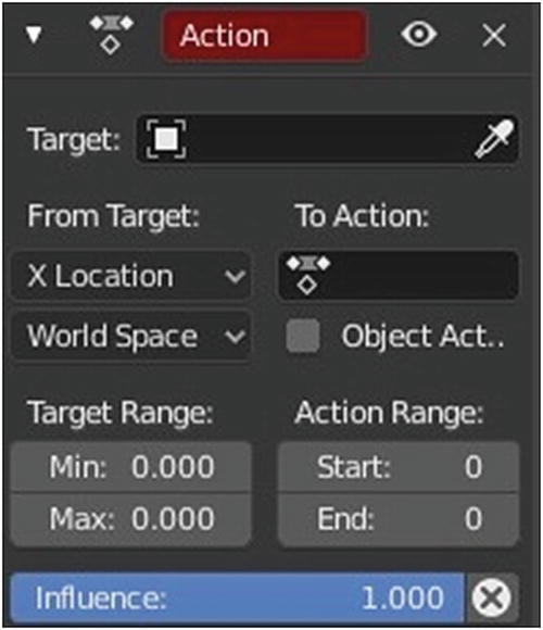
Action Constraint
Target is the data ID selects the constraints target and is not functional (red state) when it is none. Bone you can use this field when the target is an armature object. Transform Channel controls which transform property (location rotation or scale along/around one of its axes) from the target to use as action driver. Target Space allows you to choose the space to evaluate its target’s transform properties. To Action selects the name of the action you want to use. Object Action this option makes the constrained bone use the object part of the linked action instead of the same-named pose part. This allows you to apply the action of an object to a bone. Target Range Min/Max lower and upper bounds of the driving transform property value. Action Range Start/End starting and ending frames of the action to be mapped. Influence is the amount of constraint on the final solution.
Armature Constraint is the constraint version of the Armature Modifier, exactly reproducing the weight-blended bone transformations and applying it to its owner orientation. It can be used like a variant of the Child Of constraint that can handle multiple parents at once, but requires all of them to be bones.

Armature Constraint
Add Target Bone adds a new empty entry at the end of the target list. Normalize Weights normalizes all weight values in the target list so that they add up to 1.0. Preserve Volume enables the use of quaternions for preserving the volume of the object during deformation. Use Envelopes to approximate envelope-only behavior of the modifier add all relevant bones with weight 1.0. Influence is the amount of constraint on the final solution.
Child Of Constraint is the constraint version of the standard parent/children relationship between objects.
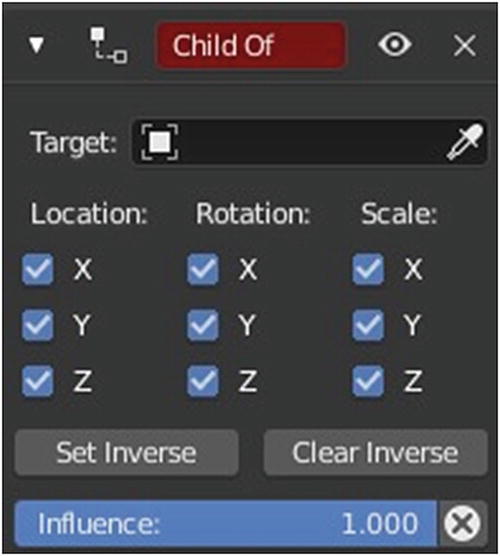
Child Of Constraint
Target the target object that this object will act as a child of. Location XYZ makes the parent affect or not affect the location along the corresponding axis. Rotation XYZ makes the parent affect or not affect the rotation around the corresponding axis. Scale XYZ makes the parent affect or not affect the scale along the corresponding axis. Set inverse restores the owner to its before-parenting state. Clear Inverse cancels the effect of set inverse and restores the owner/child to its default state regarding its target/parent. Influence is the amount of constraint on the final solution.
Floor Constraint allows you to use its target position (and optionally rotation) to specify a plane with a forbidden side, where the owner cannot go.

Floor Constraint
Targets is the data ID selects the constraints target and is not functional (red state) when it is none. Use Rotation forces the constraint to take the target’s rotation into account and allows you to have a floor plane of any orientation you like. Offset allows you to offset the floor from the target’s origin by the given number of units. Max/Min controls the plane that is the floor. Space means the standard conversion between spaces. Influence is the amount of constraint on the final solution.
Follow Path Constraint places its owner onto a curve target object, and makes it move along this curve (or path). It can also affect its owner’s rotation to follow the curve’s bends, when the Follow Curve option is enabled.

Follow Path Constraint
Targets is the data ID selects the constraints target and is not functional (red state) when it is none. Animate Path adds an F-curve with options for the start and end frame. Follow Curve if it is not activated the owner’s rotation is not modified by the curve but when activated its effect is based on the option you will select between this two: Forward axis of the object that has to be aligned with the forward direction of the path and the Up axis of the object that has to be aligned with the world z axis. Curve Radius concerns objects scaled by the curve radius. Fixed Position objects stay locked to a single point somewhere along the length of the curve regardless of time. Offset is the number of frames to offset from the animation defined by the path. Influence is the amount of constraint on the final solution.
Pivot Constraint allows the owner to rotate around a target object. It was originally intended for pivot joints found in humans e.g. fingers, feet, elbows, and so forth.
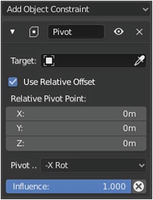
Pivot Constraint
Target is the data ID for the selection of the object to be used as a pivot point. Use relative Offset enables usage of Relative offset. Relative Pivot Point XYZ offset of pivot from target. Pivot when sets when to use the pivot. There are seven options. Always uses the pivot point in every rotation. -X Rot uses the pivot point in the negative rotation range around the x axis. -Y Rot uses the pivot point in the negative range around the y axis. -Z Rot uses the pivot point in the negative rotation range around the z axis. X Rot uses the pivot point in the positive rotation range in x axis. Y Rot uses the pivot point in the positive rotation range in y axis. Z Rot uses the pivot point in the positive rotation range in the z axis. Influence is the amount of constraint on the final solution.
Shrinkwrap Constraint is the object counterpart of the Shrinkwrap Modifier. It moves the owner origin and therefore the owner object’s location to the surface of its target.

Shrinkwrap Constraint
Target is the data ID selects the constraint’s target, which must be a mesh object, and is not functional when it has none. Distance is number field controls the offset of the owner from the shrunk computed position on the target’s surface. Shrinkwrap type allows you to select which method to use to compute the point on the target’s surface to move the owner’s origin. There are four options. Nearest Surface Point shrinks the location to the nearest target surface. Project shrinks the location to the nearest target surface along a given axis. Nearest Vertex shrinks the location to the nearest target vertex. Target Normal Project shrinks the location to the nearest target surface along the interpolated vertex normals of the target.
Snap mode allows you to choose a snapping mode for this constraint. There are five options. With Surface, the point is constrained to the surface of the target object with distance offset towards the original point location. Inside the point is constrained to be inside the target object. With Outside, the point is constrained to be outside the target object. With Outside Surface, the point is constrained to the surface of the target object with distance offset always to the outside towards or away from the original location. With Above Surface, the point is constrained to the surface of the target object with distance offset applied exactly along the target normal. Align Axis to Normal aligns the specified axis to the surface normal. Influence is the amount of constraint on the final solution.
Visit https://docs.blender.org/manual/en/latest/animation/constraints/index.html to learn more about Blender object constraints.
Particles
Particles are lots of items emitted from mesh objects, typically in the thousands. Each particle can be a point of light or a mesh, and be joined or dynamic. They may react to many different influences and forces, and have the notion of a lifespan. Dynamic particles can represent fire, smoke, mist, and other things such as dust or magic spells.
There are two types of particles: Hair and Emitter. In Hair, particles rendered as strands while in Emitter, particles are emitted in an object.
- 1.
Create the mesh that emits particles.
- 2.
Create one or more Particle Systems to emit from the mesh. Many times, multiple particle systems interact or merge with each other to achieve the overall desired effect.
- 3.
Tailor each Particle System’s settings to achieve the desired effect.
- 4.
Animate the base mesh and other particle meshes involved in the scene.
- 5.
Define and shape the path and flow of the particles.
- 6.
For Hair Particles Systems: Sculpt the emitter’s flow (cut the hair to length and comb it)
- 7.
Make the final render and do physics simulation, and tweak.
- 8.
Bake your particles.
Particle System in Properties Editor
Let’s briefly discuss each panel in each type of the Particle settings.
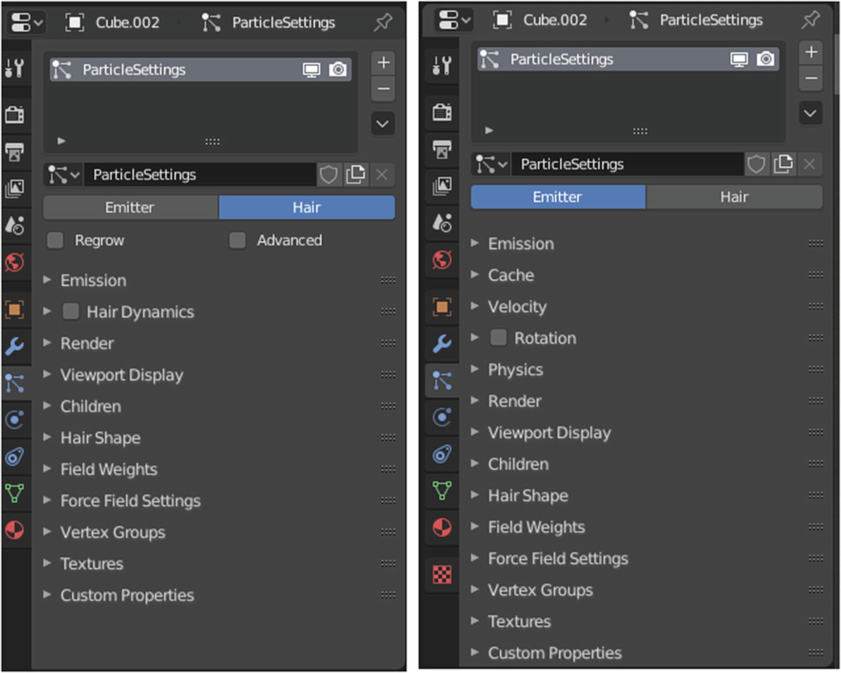
Emission Panel
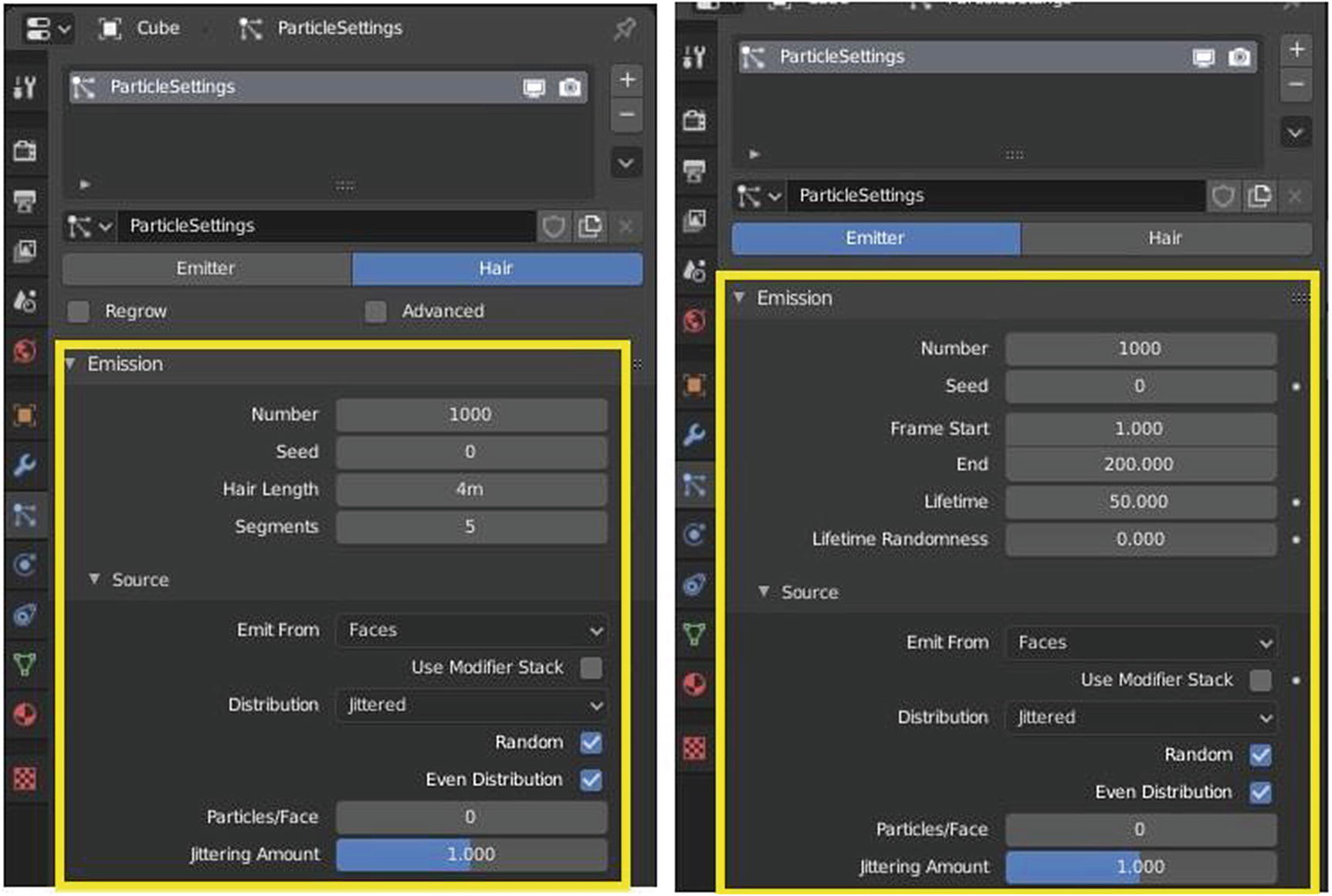
An Emitter system works like its name suggests; it emits/produces particles for a certain amount of time. In such a system, particles are emitted from the selected object from the Start frame to the End frame and have a certain lifespan. These particles are rendered as Halos, something you can see but they do not have any substance while Hair system, as its name suggested, can be used for strand-like objects, such as hair, fur, grass, quills and anything alike.
Let’s analyze the emission panel between of Hair and Emitter base on Figure 5-78. Both of them have the Number setting is the maximum number of parent particles in the simulation. Both of them have the Seed settings, which is for offset in the random number table, to get a different randomized result. Both Hair and Emitter have the Source panel inside the Emission panel. The Emit From settings are where you indicate where to emit particles from. The Distribution settings are where you indicate how to distribute particles on selected element. The Random settings are where you enable the elements to emit in random order. The Even Distribution settings are where you use even distribution from faces based on face areas or edge length. The Particles/Face settings are where you indicate emission location. The Jittering Amount settings are where you indicate the amount of jitter applied to the sampling.
Let’s talk about the differences. Hair particles have the Hair Length setting, where you can indicate the length of the hair strand. Segments settings, where you can indicate the number of hair segments. The Emitter particles have Frame Start/End settings, where you can indicate the frame number to start/end emitting particles. Lifetime settings, where you can indicate the life span of the particles. Lifetime Randomness, where you indicate the random variation of a particle life.
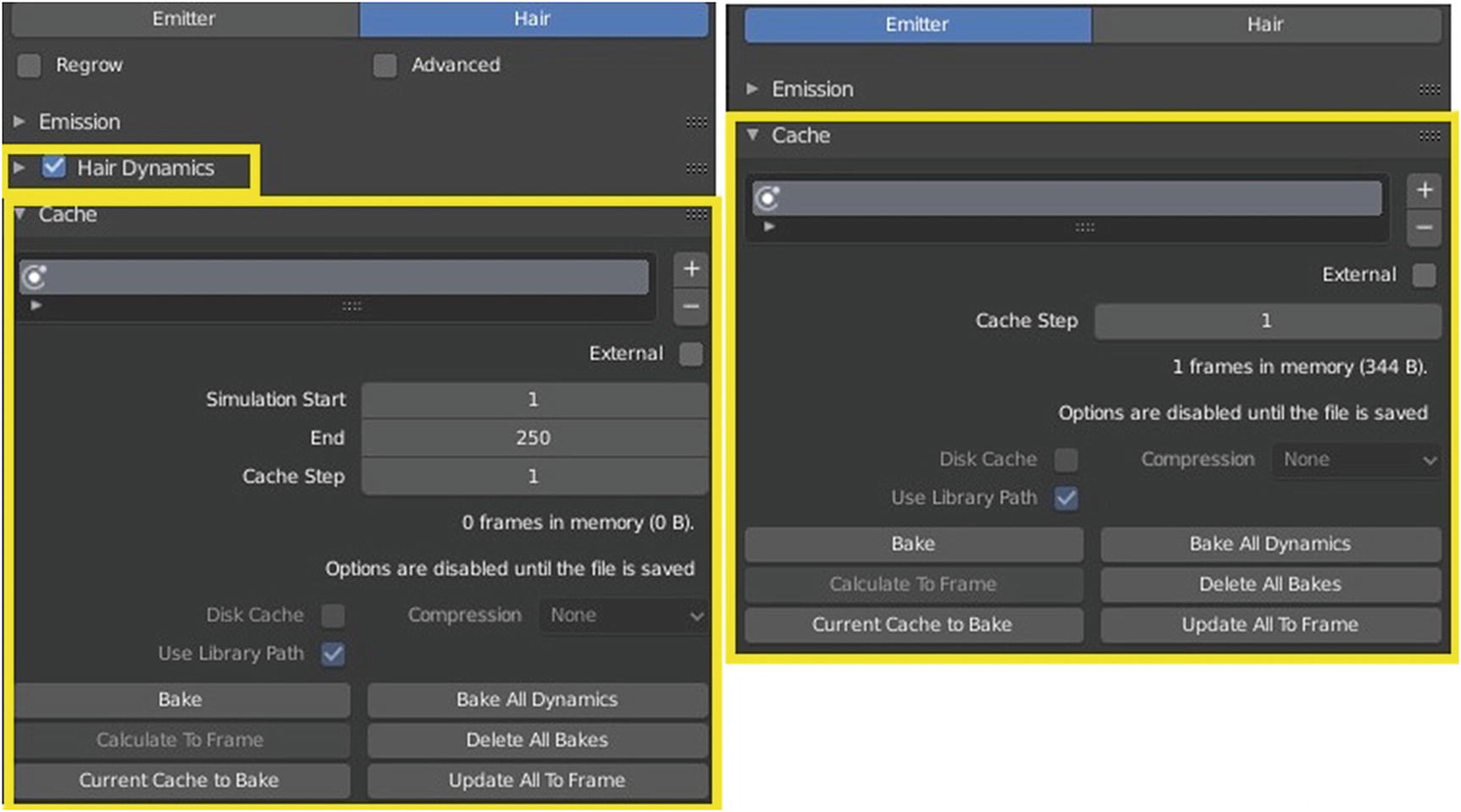
Cache Panel
By default, the Cache panel is visible in the Emitter tab, but in the Hair Particles tab, you need to enable the Hair Dynamics panel to show it.
Particle System ➤ Cache panel
They also have a lot of similar tools in this panel. They both have Cache Step, where you can indicate the number of frames between the cached frames. They also both have that long rectangle where you can see the list of cache, where you can rename it, add a cache, and delete one. They both can access to external location to read cache file by enabling the External setting. They also have Bake/Calculate to Frame button for bake physics, Current Cache to Bake button to bake the cache, Bake All Dynamics/Update All to Frame button, which is used for baking all physics. Delete All Bakes deletes all baked caches of all objects in the current scenes.
Hair particles have Simulation start/end settings, where you can indicate on which frame the simulation starts and ends.
Note
The simulation is only calculated for positive frames between the Start and End frames of the Cache panel, whether you bake or not. So if you want a simulation that is longer than the default frame range, you have to change the End frame. When animation is played, the physics writes each frame to the cache. For the cache to fill up, one has to start the playback before or on the frame that the simulation starts. The cache is cleared automatically on changes. But not on all changes, so it may be necessary to free it manually. The system is protected against changes after baking. If the mesh changes the simulation is not calculated as anew, the bake result can be cleared by clicking the Free Bake button on the simulation cache settings. A simulation can only be edited in Particle mode when it has been baked to a Disk Cache. If you are not allowed to write to the required subdirectory caching will not take place. Be careful with the sequence of modifiers in the modifier stack. You may have a different number of faces in the 3D Viewport and for rendering. If so, the rendered result may be very different from what you see in the 3D Viewport.
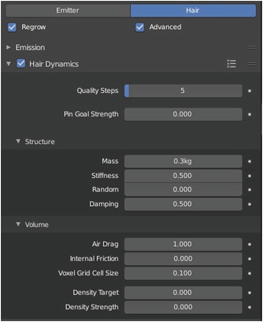
Hair Dynamics
Hair Dynamics is used for greater enhancement of hair particles or for animating hair particles.
Hair Particle System ➤ Hair Dynamics panel
Quality Steps indicates the quality of the simulation in steps per frame. The Pin Goal Strength indicates pin spring stiffness. In Structure, Mass indicates the mass of cloth material. Stiffness indicates how much the material resists bending. Random indicates random stiffness in the hair. Damping indicates the amount of damping in bending behavior.
Air Drag indicates the thickness of the air that makes things falls slowly. Internal friction indicates the number of friction of hair volume. Voxel Grid Cell Size indicates the size of the voxel grid cells for interaction effects. Density Target indicates maximum hair density and Density Strength indicates the influence of target density on the simulation.
Note
A voxel represents a value on a regular grid in 3D space. Voxel grid is a 3D grid. A collection of aligned boxes.
Velocity Panel
When it comes to Hair Particles, Velocity panel, as well as Rotation and Physics, only appears when you check the Advanced option at the top of the Hair Particles settings.

Particle System ➤ Velocity panel
When it comes to Hair Particles, Velocity panel, as well as Rotation and Physics, only appears when you check the Advanced option at the top of the Hair Particles settings.
Both Particles have the same settings for this panel. Normal lets the surface normal give the particle a starting velocity. Tangent lets the surface tangent give the particle a starting velocity. Tangent Phase rotates the surface tangent. Object Aligned lets the emitter object orientation give the particle a starting velocity. Object Velocity lets the object give the particle a starting velocity. Randomize gives the stating velocity a random variation.
Rotation Panel
Rotation panel have these tools: Orientation Axis sets the initial orientation of the particle. Randomize allows you to randomize particle orientation. Phase sets the rotation around the chosen axis. Randomize Phase where you can randomize the rotation around the chosen axis. The Axis settings allow you to choose which axis changes the particle rotation in time. The Amount settings are for the angular velocity amount. When the Dynamic tool in Emitter is enabled, the particles rotation is affected by collision and effectors.

Particle System ➤ Rotation panel
Physics Panel

Particle System ➤ Physics panel
Physics Type is where you can choose particles physics type. In Physics Type, there are five options: None, Newtonian, Keyed, Fluids, and Boids. Mass indicates the mass of the particles. Forces lets you see the settings of Brownian, where you can specify the amount of Brownian motion that adds random motion to the particles based on a Brownian noise field. Brag specifies the amount of force that reduces particles velocity in relation to its speed and size. Damp specifies the amount of reduces particle velocity.
Render Panel
Render As specifies how particles are rendered. There are four options for Hair Particles: None, Path, Object, and Collection. There are six options for Emitter: Collection, Object, Path, Line, Halo, and None. By default, Halo is set in Emitter while Path is set in Hair Particles. Material is a material slot for particle system. Both of them have Coordinate System specifies an object’s coordinate system and Path sets B-Spline is for interpolation. Steps specifies the number of steps that paths are rendered with. Timing specifies the end time of drawn path through End settings, where you can give path length a random variation through Random settings.
Emitter Particles have two settings in the Render panel that are not available in Hair Particles. These are Scale where you can specify the size of the particles and Scale Randomness where you can give the particle size a random variation.
There are other functions, but I will not cover them.

Particle System ➤ Render panel
Viewport Display Panel
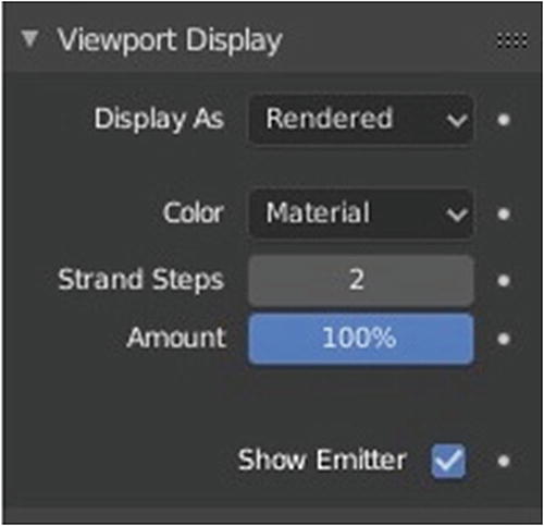
For this panel, both particles have the same settings. Display As is where you choose how particles are drawn in viewport. There are six options on the Emitter tab: None, Rendered, Point, Circle, Cross, and Axis. There are three options on the Hair Particles tab: None, Rendered and Path. The default option set for both Emitter and Hair is Rendered. The Color setting is where you can choose where to draw additional particle data as color. There are four options: None, Material (default), Velocity, and Acceleration. Strand Steps is where you specify how many steps paths are drawn with while Amount is where you specify the percentage of particles to display in the 3D Viewport. Enabling Show Emitter makes the instancer visible in the viewport or the mesh that the particles are emitting from.
Children Panel
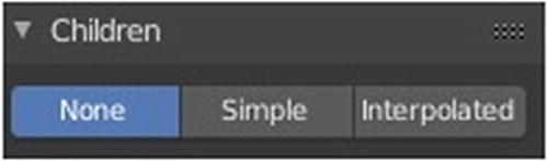
Particle System ➤ Children panel
In this panel, both the Emitter and Hair particles have the same settings.
In this panel is where you can set the creation of child particles. As you can see in Figure 5-86, there are three options: None, Simple, and Interpolated. None means that no children are generated. Simple means that children are emitted from the parent position. Interpolated means that children are emitted between the Parents particles on the faces of a mesh. They interpolate between adjacent parents. This is especially useful for fur, because you can achieve an even distribution.
Hair Shape Panel

Particle System ➤ Hair Shape panel
This panel can be seen in both Emitter and Hair particles. Strand Shape specifies the strand shape parameter. Radius Root specifies the strand with at the root. Tip specifies the strand width at the tip. Radius Scale specifies the multiplier of radius properties. Close Tip sets the tip radius to 0.
Field Weights Panel
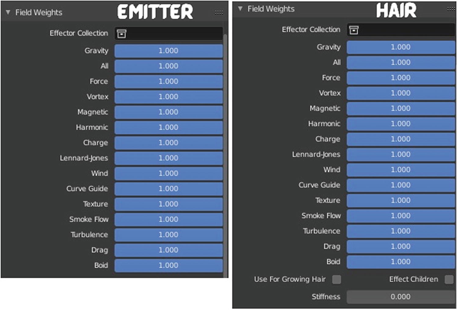
Particle System ➤ Field Weights panel
In this panel, the two particles settings have few differences. Let’s talk first about the common settings.
Gravity specifies the global gravity weight. All specifies all effectors’ weights. Force specifies the force effector weight. Vortex specifies the vortex effector weight. Magnetic specifies the magnetic effector weight. Harmonic specifies the harmonic effector weight. Charge specifies the charge effector weight. Lennard-Jones specifies the Lennard-Jones effector weight. Wind specifies the wind effector weight. Curve Guide specifies the Curve Guide effector weight. Texture specifies the texture effector weight. Smoke Flow specifies the Smoke Flow effector weight. Turbulence specifies the turbulence effector weight. Drag specifies the drag effector weight. Boid specifies the Boid effector weight.
In the Hair particle settings, Stiffness specifies the hair stiffness for effectors. Use for Growing Hair applies force fields when growing hair. Effect Children applies effectors to children.
Force Field Settings Panel

Particle System ➤ Force Field Settings panel
Both particles have the same settings in this panel. Self Effect makes particles effectors affect Effector Amount. Type1 is the type of field. There are 14 options: Smoke Flow, Drag, Turbulence, Boid, Curve Guide, Texture, Lennard-Jones, Charge, Harmonic, Magnetic, Vortex, Wind, and Force. The settings that appear on Falloff depend on your choice in Type1. Type2 has the same settings as Type1. This is for another option of field type.
Vertex Groups Panel

Particle System ➤ Vertex Groups panel
The panel’s settings are the same for both particles.
Vertex Groups tag the vertices belonging to parts of a Mesh Objects or Lattice. Think of the legs of a chair or the hinges of a door, or hands, arms, limbs, head, feet, and so forth, of a character. In addition, you can assign different weight values to the vertices within a vertex group. Hence, vertex groups are sometimes also called weight groups.
Density controls the density. Length controls the length. Clump controls the clump. Kink controls the kink. Roughness1/2 controls the roughness. Roughness End controls the roughness end. Twist controls the twist.
The arrow beside the rectangle is to negate the effect of the given effect to the vertex group; for example, the density.
Textures Panel
Textures are like additional layers on top of base material. Textures affect one or more aspects of the object’s net coloring. The net color you see is a sort of layering effects.

Particle System ➤ Textures panel
Physics
Blender’s Physics system allows you to simulate a number of different real-world physical phenomena. You can use these systems to create a variety of static and dynamic effects.
There are nine types of physics: Force Field, Collision, Cloth, Dynamic Paint, Soft Body, Fluid, Smoke, Rigid Body, and Rigid Body Constraint. Let’s briefly discuss each.
Force Field Physics
Force Field offers a way to influence a simulation, in example to add extra movement. Particles, Soft Bodies, Rigid Bodies, and Cloth objects can all be affected by forces fields. Force fields automatically affect everything.
Its settings depend on which Type you choose. The Shape type sets the direction to calculate the effector force. There are 13 options available: Force (default), Wind, Vortex, Magnetic, Harmonic, Charge, Lennard-Jones, Texture, CurveGuide, Boid, Turbulence, Drag, and Smoke Flow.
There are types that have the same settings, and there are types that have only small differences.
Force Field Type ➤ Boid, Charge, Lennard-Jones, Magnetic, Wind Force, and Vortex
The settings for Boid, Charge, Lennard-Jones, Magnetic, and Wind are the same, but the application of these types is different. The settings of these five types have a lot of similarities to Force and Vortex settings too. So let’s discuss its functions.
Boid is an artificial life program developed by Craig Reynolds in 1986. It simulates the flocking behavior of birds. The rules applied in the simplest Boids world are as follows.
Separation steers to avoid crowding local flock mates. Alignment: steer towards the average heading of local flock mates. Cohesion steers to move toward the average position of local flock mates. Complex rules can be added, such as obstacle avoidance and goal seeking.
Charge is similar to a Force type except it changes it’s behavior based on the effected particles charge field, which means that this field has only an effect on particles that have also a Charge field.
Lennard-Jones is a very short range force with a behavior determined by the sizes of the effector and effected particles. At a distance smaller than the combined sizes, the field is very repulsive, but after that distance, it is attractive. It tries to keep the particles at an equilibrium distance from each other. Particles need to be at a close proximity to each other to be effected by this field at all.
Magnetic depends on the speed of the particles. It simulates the force of magnetism on magnetized objects.
Wind gives a constant force in a single direction, along the force object’s local z axis. The strength of the force is visualized by the spacing of the circles.
Force is the simplest of the fields. It gives a constant force toward (positive strength) or away from (negative strength) the object’s origin. Newtonian particles are attracted to a field with negative strength, and are blown away from a field with positive strength.
Vortex gives a spiraling force that twists the direction of points around the force object’s local z axis. This can be useful for making a swirling sink, or a tornado, or kinks in particle hair.

Magnetic (represents the settings of Lennard-Jones, Wind, Charge, and Boid), Force, Vortex
- Shape. Sets the direction to calculate the effector force.
Point. Points with omni-directional influence. Uses the object origin as the effector point.
Line (not part of Vortex Field). Field originates from the local z axis of the object.
Plane. Influences only in the local Z direction.
Surface (not part of Vortex Field). The force fields act on a 3D object’s surface. In this case, the z axis is the surface normal.
Every Point. Uses every vertex in the mesh object as an effector point.
Surface Falloff. Can only be found in the Vortex field.
Strength. The strength of the force field.
Flow. Convert effector force into air flow velocity.
Affect Location. Affects particle location.
Affect Rotation. Affects particle dynamic rotation.
Noise Amount. The amount of noise for the force strength.
Seed. Seed of the noise.
Gravitation (Force Field only). Multiply force by 1/distance2.
Absorption. Force is absorbed by collision objects.
- Shape. Falloff type.
Sphere. The falloff is uniform in all directions.
Tube. The falloff results in a tube-shaped force field.
Cone. The falloff results in a cone-shaped force field.
- Z Direction. Effect in full or only positive/negative Z direction. There are three options for this one.
Both Z
Z+
Z-
Power. How quickly strength falls off with distance from the force field.
Use minimum. Use a minimum distance for the field’s fall off.
Min Distance. Minimum distance for the field’s fall off.
Use maximum. Use a maximum distance for the field to work.
Force Field Type ➤ Harmonic and Turbulence
These two have almost the same settings with each other. They only have a few differences.
In Harmonic, the source of the force field is the zero point of a harmonic oscillator. If you set the Damping parameter to 1, the movement is stopped in the moment the object is reached. This force field is really special if you assign it to particles.
Turbulence creates a random and chaotic 3D noise effect, similar to jets of water or geysers under the ocean.

Harmonic and Turbulence
- Shape. Sets the direction that calculates the effector force.
Point. Point with omni-directional influence. Uses the object origin as the effector point.
Line. Field originates from the local z axis of the object.
Plane. Influence only in the local Z direction.
Surface. The force fields act on a 3D object’s surface. In this case, the z axis is the surface normal.
Every Point. Uses every vertex in the mesh object as an effector point.
Strength. The strength of the force field.
Flow. Convert effector force into air flow velocity.
Damping (Harmonic). Damping of the harmonic force.
Rest Length (Harmonic). Rest length of the harmonic force.
Size (Turbulence). Size of the Turbulence.
Affect Location. Affects particle location.
Affect Rotation. Affects particle dynamic rotation.
Noise Amount. The amount of noise for the force strength.
Seed. Seed of the noise.
Multiple Springs (Harmonic). Every point is affected by multiple strings.
Global (Turbulence). Use effector/global coordinates for Turbulence.
Absorption. Force is absorbed by collision objects.
- Shape. Falloff type.
Sphere. The falloff is uniform in all directions.
Tube. The falloff results in a tube-shaped force field.
Cone. The falloff results in a cone-shaped force field.
- Z Direction. Effect in full or only positive/negative Z direction. There are three options for this one.
Both Z
Z+
Z-
Power. How quickly strength falls off with distance from the force field.
Use minimum. Use a minimum distance for the field’s fall off.
Min Distance. Minimum distance for the field’s fall off.
Use maximum. Use a maximum distance for the field to work.
Force Field Type ➤ Curve Guide
This forces particles to follow a certain path defined by a Curve Object. A typical scenario would be to move a red blood cell inside a vein, or to animate the particle flow in a motor. You can also use Curve Guide to shape certain hair strands.
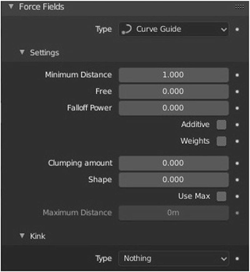
Curve Guide
Minimum Distance. The distance from which particles are affected fully.
Free. Guide-free time from particle life’s end.
Falloff Power. How quickly strength falls off with distance from the force field.
Additive. Based on distance/falloff it adds a portion of the entire path.
Weights. Use curve weights to influence the particle influence along the curve.
Clumping Amount. The amount of clumping.
Shape. Shape of clumping.
Use Max. Use a minimum distance for the field to work.
Maximum Distance. Maximum distance for the field to work.
Type. The type of periodic offset on the curve. There are seven options for this kink: Roll, Rotation, Braid, Wave, Radial, Curl, and Nothing, which is the default value.
Force Field Type ➤ Drag
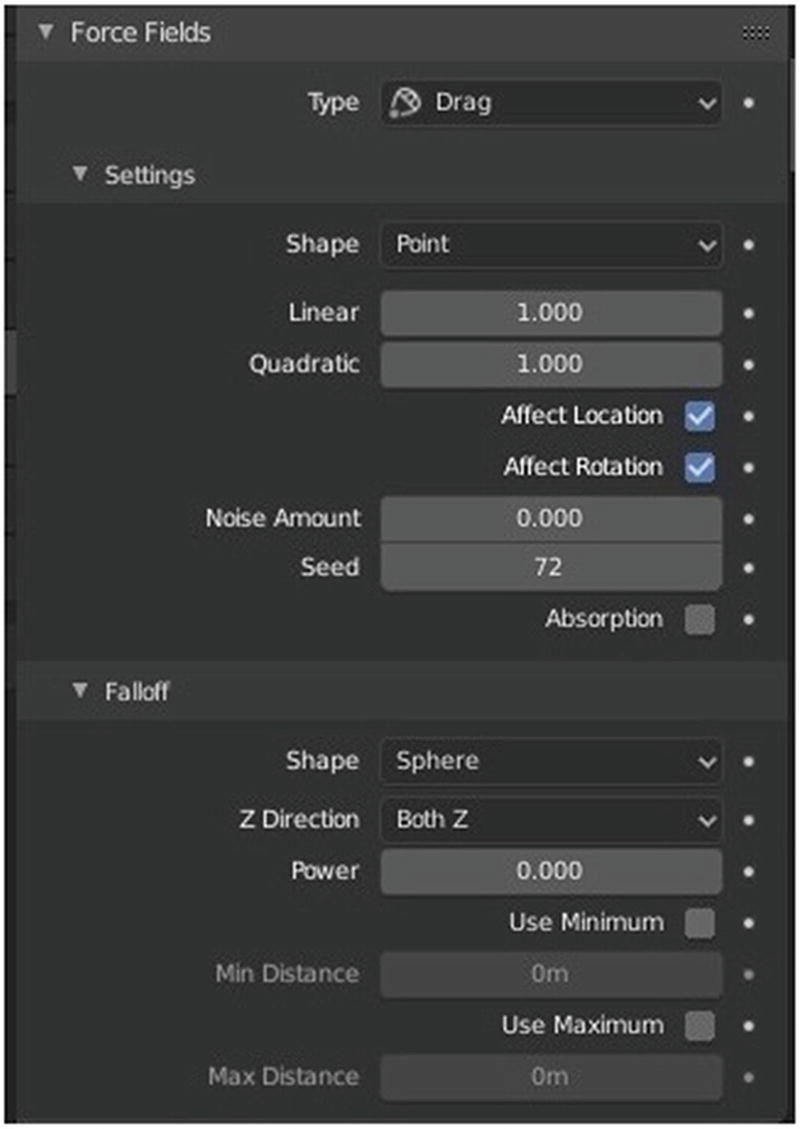
Drag
- Shape. Sets the direction to calculate the effector force.
Point. Point with omni-directional influence. Uses the object origin as the effector point.
Line. Field originates from the local z axis of the object.
Plane. Influence only in the local Z direction.
Surface. The force field acts on a 3D object’s surface. In this case, the z axis is the surface normal.
Every Point. Uses every vertex in the mesh object as an effector point.
Linear. Drag component proportional to velocity.
Quadratic. Drag component proportional to the square of velocity.
Affect Location. Affects particle location.
Affect Rotation. Affects particle dynamic rotation.
Noise Amount. The amount of noise for the force strength.
Seed. Seed of the noise.
Absorption. Force is absorbed by collision objects.
- Shape. Falloff type.
Sphere. The falloff is uniform in all directions.
Tube. The falloff results in a tube-shaped force field.
Cone. The falloff results in a cone-shaped force field.
- Z Direction. Effect in full or only positive/negative Z direction. There are three options for this one.
Both Z
Z+
Z-
Power. How quickly strength falls off with distance from the force field.
Use minimum. Use a minimum distance for the field’s fall off.
Min Distance. Minimum distance for the field’s fall off.
Use maximum. Use a maximum distance for the field to work.
Force Field Type ➤ Texture
You can use a Texture force field to create an arbitrarily complicated force field, which force in the three directions is color coded. Red is coding for the x axis, green for the y axis, and blue for the z axis (like the color of the coordinate axes in the 3D View).

Texture
Texture mode. How the texture effect is calculated. There are three options: RGB, Curl, and Gradient.
Strength. The strength of the force field.
Nabla. Defines size of derivative offset used for calculating gradient and curl.
Use Coordinates. Use object/global coordinates for texture.
2D. apply force only in 2D.
Checkered icon drop-down button. Browse texture to be linked.
New button. Add new texture.
- Shape. Falloff type.
Sphere. The falloff is uniform in all directions.
Tube. The falloff results in a tube-shaped force field.
Cone. The falloff results in a cone-shaped force field.
- Z Direction. Effect in full or only positive/negative Z direction. There are three options for this one.
Both Z
Z+
Z-
Power. How quickly strength falls off with distance from the force field.
Use minimum. Use a minimum distance for the field’s fall off.
Min Distance. Minimum distance for the field’s fall off.
Use maximum. Use a maximum distance for the field to work.
Force Field Type ➤ Smoke Flow
This force field type creates a force based on a Smoke simulation air flow. It applies the smoke simulation air flow velocity as a force to other simulations that use force fields.
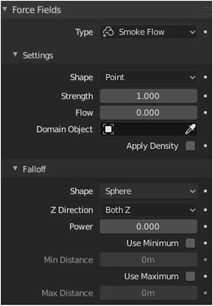
Smoke Flow
- Shape. Sets the direction to calculate the effector force.
Point. Point with omni-directional influence. Uses the object origin as the effector point.
Line. Field originates from the local z axis of the object.
Plane. Influences only in the local Z direction.
Surface. The force field acts on a 3D object’s surface. In this case, the z axis is the surface normal.
Every Point. Uses every vertex in the mesh object as an effector point.
Strength. The strength of the force field.
Flow. Converts effector force into air flow velocity.
Domain Object. Selects domain object of the smoke simulation.
Apply Density. Adjust force strength based on smoke density.
- Shape. Falloff type.
Sphere. The falloff is uniform in all directions.
Tube. The falloff results in a tube-shaped force field.
Cone. The falloff results in a cone-shaped force field.
- Z Direction. Effect in full or only positive/negative Z direction. There are three options for this one.
Both Z
Z+
Z-
Power. How quickly strength falls off with distance from the force field.
Use minimum. Use a minimum distance for the field’s fall off.
Min Distance. Minimum distance for the field’s fall off.
Use maximum. Use a maximum distance for the field to work.
Collision Physics
There are two different collision types that you may use: collision between different objects and internal collision. We should set one thing straight from the start: the primary targets of the collision calculation are the vertices of a soft body. So if you have too few vertices, too few collisions take place. Also, you can use edges and faces to improve the collision calculation.

Collision
Field Absorption. The percentage of effector force that is lost during a collision with this object.
Particle ➤ Permeability. Chance that the particle passes through the mesh.
Particle ➤ Stickiness. The amount of stickiness to surface collision.
Particle ➤ Kill Particles. Kill collided particles.
Particle ➤ Damping. The amount of damping during particle collision.
Particle ➤ Randomize. Random variation of damping.
Particle ➤ Friction. The amount of friction during particle collision.
Particle ➤ Randomize. Random variation of friction.
Softbody and Cloth ➤ Damping. The amount of damping during softbody and cloth collision.
Softbody and Cloth ➤ Thickness Outer/Inner. The amount of outer/inner thickness.
Softbody and Cloth ➤ Friction. Friction of cloth collision.
Cloth Physics
Cloth simulation is one of the hardest aspects of CG, because it is a deceptively simple real-world item that is taken for granted, yet actually has very complex internal and environmental interactions. After years of development, Blender has a very robust cloth simulator that makes clothing, flags, banners, and so on. Cloth interacts with and is affected by other moving objects, the wind and other forces, and a general aerodynamic model—all of which is under your control.
A piece of cloth is any mesh, open or enclosed, that has been designated as cloth. The Cloth panels are located in the Physics tab and consist of three panels of options. Cloth is either an open or closed mesh and is mass-less, in that all cloth is assumed to have the same density, or mass per square unit.

Cloth
Quality Steps. Quality of the simulation in steps per frame.
Speed Multiplier. Cloth speed is multiplied by this value.
Physical Properties ➤ Mass. Mass of cloth material.
Physical Properties ➤ Air Viscosity. Air has normally thickness that slows falling things.
Physical Properties ➤ Bending Model. Physical model for simulating bending forces. There are two types: Angular and Linear.
Stiffness ➤ Tension. How much the material resists stretching. This is not present when Bending model is set to Linear.
Stiffness ➤ Compression. How much the material resists compression.
Stiffness ➤ Shear. How much the material resists shearing.
Stiffness ➤ Bending. How much the material resists bending.
Damping ➤ Tension. The amount of damping in stretching behavior. This is not present when Bending model is set to Linear.
Damping ➤ Compression. The amount of damping in compression behavior.
Damping ➤ Shear. The amount of damping in shearing behavior.
Damping ➤ Bending. The amount of damping in bending behavior.
Shape ➤ Pin Group. Vertex group for pinning of vertex.
Shape ➤ Stiffness. Specifies the pin spring stiffness.
Shape ➤ Sewing. Pulls loose edges together.
Shape ➤ Max Sewing Force. Specifies the maximum sewing force.
Shape ➤ Shrinking Factor. Factor by which to shrink cloth.
Shape ➤ Dynamic Mesh. Make simulation respect deformations in the base mesh.
Collision ➤ Quality. Specifies the number of collision iterations that should be done.
Object Collision ➤ Distance. Specifies the minimum distance between collision objects before collision response takes effect.
Object Collision ➤ Impulse Clamping. Specifies clamp collision impulses to avoid instability.
Object Collision ➤ Collision Collection. Where you can limit colliders.
Self Collision ➤ Friction. Specifies friction with self contact.
Self Collision ➤ Distance. Minimum distance between cloth faces before collision response takes effect.
Self Collision ➤ Impulse Clamping. Clamp collision impulses to avoid instability.
Self Collision ➤ Vertex Group. Specifies the vertex group to define vertices that are not used during self collisions.
Property Weights ➤ Structural Group. Vertex group for fine control over structural stiffness.
Property Weights ➤ Max Tension. Specifies the maximum tension stiffness value.
Property Weights ➤ Max Compression. Specifies the maximum compression stiffness value.
Property Weights ➤ Shear Group. Vertex group for fine control over shear stiffness.
Property Weights ➤ Max Shearing. Specifies the maximum shear scaling value.
Property Weights ➤ Bending Group. Vertex group for fine control over bending stiffness.
Property Weights ➤ Max Bending. Specifies the maximum bending value.
Property Weights ➤ Shrinking Group. Vertex group for shrinking cloth.
Property Weights ➤ Max Shrinking. Specifies the maximum amount to shrink by.
Dynamic Paint Physics
Dynamic Paint is a modifier and physics system that can turn objects into paint canvases and brushes, creating vertex colors, image sequences, or displacement. This makes many effects possible like, for example footsteps in the snow, raindrops that make the ground wet, paint that sticks to walls, or objects that gradually freeze.

Dynamic Paint
Format. Where you can choose a format for Dynamic paint. There are two options: Vertex and Image Sequence.
Anti-Aliasing. Use 5x multi sampling to smooth paint edges.
Frame Start. Indicates the staring frame.
Frame End. Indicates the ending frame.
Frame Sub-steps. Extra frames between scene frames to ensure smooth motion.
Subsurface Type. Choose surface type. There are four options: Paint, Displace, Weight, and Waves.
Brush Collection. Collections of brush objects.
Scale Influence. Adjust influence brush objects have on this surface.
Radius. Adjust radius of proximity brushes or particles for this surface.
Soft Body Physics
Soft Body simulates soft, deformable objects. It was designed primarily for adding secondary motion to animation, like jiggle for the body parts of a moving character.
The simulation works by combining existing animation on the object with forces acting on it. There are exterior forces like gravity or force fields and interior forces that hold the vertices together. This way you can simulate the shapes that an object would take on in reality if it had volume, was filled with something, and was acted on by real forces.
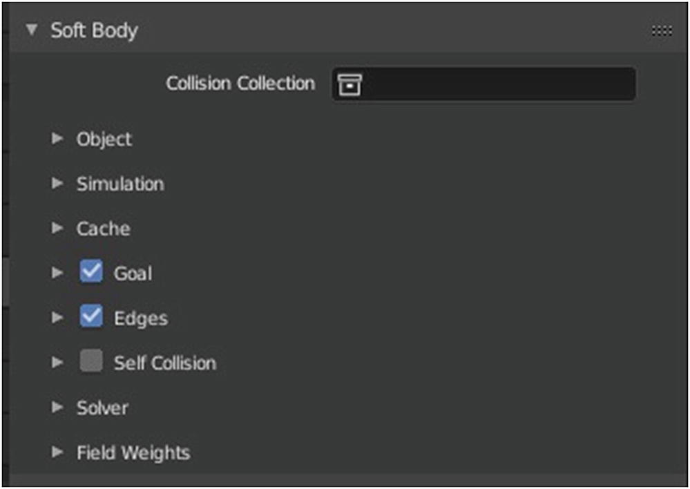
Soft Body
Object ➤ Friction. Specifies the general media friction for point movements.
Object ➤ Mass. Specifies the general mass value.
Object ➤ Control Point. Specifies the control point mass values.
Simulation ➤ Speed. Specifies the tweak timing for physics to control frequency and speed.
Goal ➤ Vertex Group. Specifies the control point weight values.
Edges ➤ Springs. Specifies the control point spring strength values.
Edges ➤ Pull. Specifies the edge spring stiffness when longer than rest length.
Edges ➤ Push. Specifies the edge spring stiffness when shorter than rest length.
Edges ➤ Length. Specifies the alter spring length to shrink/blow up. 0 to disable.
Edges ➤ Collision Edge. Edges collide too.
Edges ➤ Face. Faces collide too.
Edges ➤ Damp. Specifies the edge spring friction.
Edges ➤ Plastic. Specifies the permanent deform.
Edges ➤ Blending. Specifies the bending stiffness.
Self collision ➤ Calculation Type. Where you can choose collision type.
Self Collision ➤ Ball Size. Specifies the absolute ball size or factor if not manually adjusted.
Self Collision ➤ Stiffness. Specifies the ball inflating pressure.
Self Collision ➤ Dampness. Specifies the blending to inelastic collision.
Solver ➤ Step Size min/max. Specifies the minimal/maximum number solver steps/frame.
Solver ➤ Auto-step. Use velocities for automatic step sizes.
Solver ➤ Error Limit. Specifies the Runge-Kutta ODE solver error limit; low values give more precision; high values give speed.
Fluid Physics
Fluid Physics simulate the physical properties of liquids especially water. While creating a scene in Blender, certain objects can be marked to participate in the fluid simulation. These can include but not limited to, being a fluid or as an obstacle. For a fluid simulation you have to have a domain to define the space that the simulation takes up. In the Domain settings, you can define the global simulation parameters (such as viscosity and gravity).
Fluid has seven types: Domain, Fluid, Obstacle, Inflow, Outflow, Control, and Particle. Let’s briefly discuss the settings for each type.
Fluid ➤ Domain
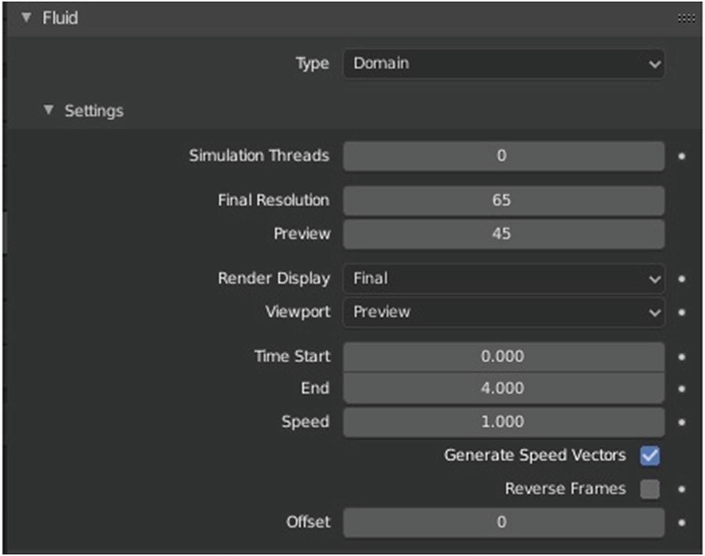
Fluid Physics ➤ Domain Type
Simulation Threads. Override number of threads for the simulation.
Final Resolution. Domain resolution in X, Y, and Z direction.
Preview. Specifies the preview resolution in X, Y, and Z direction.
Render Display. Where you can choose how to display the mesh for rendering.
Viewport. Where you can choose how to display the mesh in the viewport.
Time Start/End. Specifies the simulation time of the first/last blender frame in seconds.
Speed. Specifies the fluid motion rate.
Generate Speed Vectors. Generates speed vectors for vector blue.
Reverse Frames. Reverses fluid frames.
Offset. Specifies the offset when reading baked cache.
Fluid ➤ Outflow
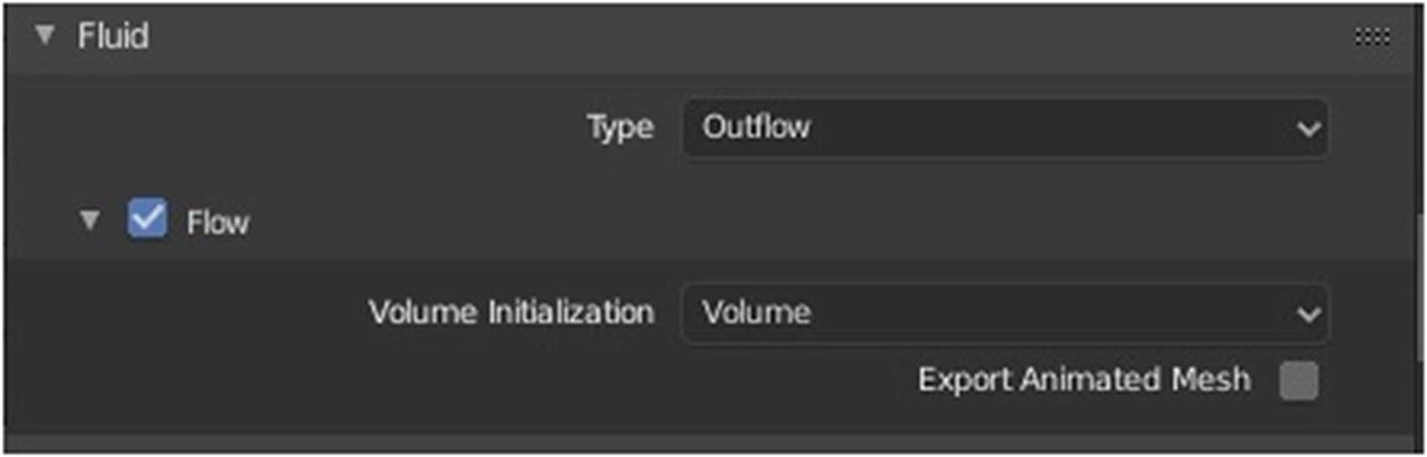
Fluid Physics ➤ Outflow Type
When you enable Flow, objects contribute to the fluid simulation. Volume Initialization is for common options among the different fluid types. There are three options. When you use Volume, the inside of the object is initialized as fluid all. This works only if the mesh is closed. When you use Shell, it is initialized as a thin fluid of the surface of the mesh. This can also be used if the mesh is open. Both can only be used in closed mesh and a mix of Volume and Shell. Export Animated Mesh exports the mesh as an animated one.
Fluid ➤ Control Type

Quality is used for object sampling. Reverse Frames reverses the control of the object movement. Time Start and End specifies the time when the control particles are activated and deactivated. Attraction Strength specifies the force strength for directional attraction towards the control object. Radius specifies the force field radius around the control object. Velocity Strength specifies how much of the control object’s velocity is influencing the fluid velocity. Radius specifies the force field radius around the control object.
Fluid ➤ Fluid

In Figure 5-105, Fluid type has settings similar to Outflow. These are Volume Initialization and Export Animated Mesh.
Initial Velocity is for the speed of the fluid at the beginning of the simulation (in meters per second).
Fluid ➤ Particle
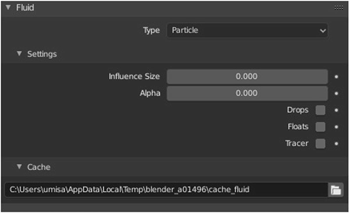
Fluid Physics ➤ Particle Type
Influence Size specifies the amount of particle size scaling. Alpha specifies the amount of particle alpha changes. With Drops, surface splashes of the fluid result in droplets being strewn about, like fresh water, with low Surface Tension. With Floats, the surface tension of fluid is higher and the fluid heavier, like cold seawater and soup. Breakaways are clumpier and fall back to the surface faster than Drops as with high Surface Tension. With Tracer, droplets follow the surface of the water where it existed, like a fog suspended above previous fluid levels.
Fluid Type ➤ Inflow
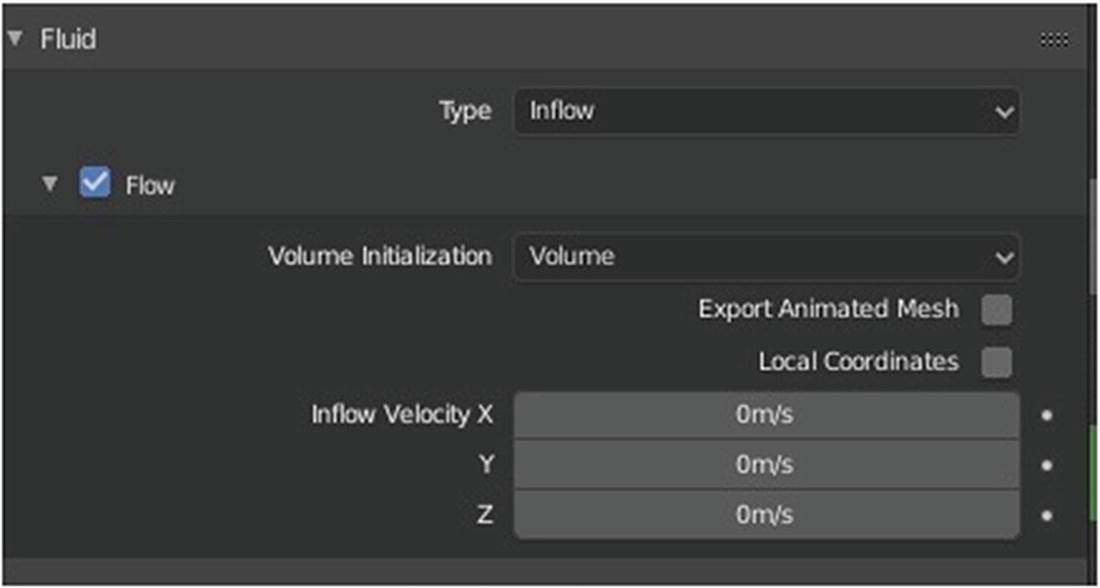
Fluid Physics ➤ Inflow Type
In Figure 5-107, the Inflow settings are the same as Fluid Type. These are Volume Initialization, Exported Animated Mesh, and Initial Velocity, which is called Inflow Velocity.
When you enable Local Coordinates, it uses local coordinates for inflow.
Fluid Type ➤ Obstacle Type
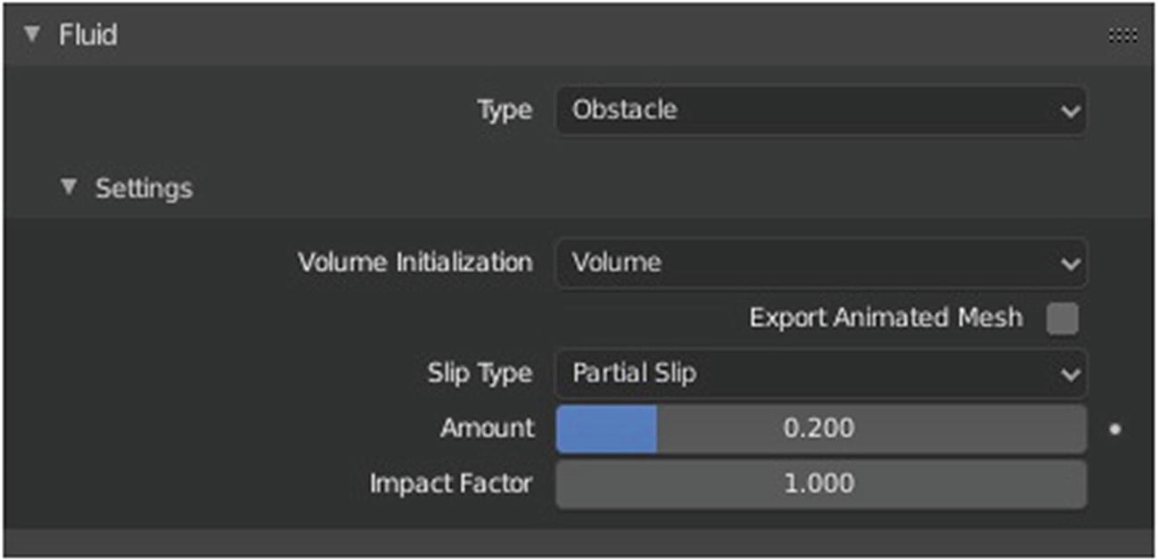
Fluid Physics ➤ Obstacle Type
The Slip Type setting is for the stickiness of the surface of the obstacle, to determine the tacky-surface. There are three options: Partial Slip (the default), No Slip, and Free Slip. Amount is where you specify the amount of mixing between no and free slip. 0 is no slip and 1 is free slip. Impact Factor is where you specify the value that controls the impact an obstacle has on the fluid. Making it zero behaves like outflow while greater than one results in high forces. One is the default.
Smoke Physics
Smoke simulation is a subset of the fluid system, can be used for simulating collections of airborne solids, liquid particulates, and gases, such as those that make up smoke. It simulates the fluid movement of air and generates animated voxel textures representing the density, heat, and velocity of other fluids or suspended particles that can be used for rendering.
Smoke Simulation have three types: Domain, Flow, and Collision. Each have their own settings.
Smoke ➤ Domain Type

Smoke Simulation Physics ➤ Domain Type
Resolution Divisions. Specifies the maximal resolution used in the fluid domain.
Time Scale. Adjust simulation speed.
Border Collisions. Where you select the domain border is treated as collision object.
Empty Space. Value under which voxels are considered empty space to optimize caching and rendering.
Behavior ➤ Density. How much density affects smoke motion.
Behavior ➤ Temperature Difference. How much heat affects smoke motion.
Behavior ➤ Vorticity. The amount of turbulence/rotation in fluid.
Dissolve ➤ Time. Dissolving speed.
Adaptive Domain ➤ Add Resolution. Maximum number of additional cells.
Adaptive Domain ➤ Margin. Specifies the margin added around fluid to minimize boundary interference.
Adaptive Domain ➤ Threshold. Specifies the maximum amount of fluid cell can contain before it is considered empty.
Flames ➤ Reaction Speed. Specifies the speed of the burning reaction.
Flames ➤ Smoke. Specifies the amount of smoke created by burning fuel.
Flames ➤ Vorticity. Specifies the additional vorticity for the flames.
Flames ➤ Temperature Ignition. Specifies the minimum temperature of flames.
Flames ➤ Maximum. Specifies the maximum temperature of flames.
Flames ➤ Smoke Color. Specifies the color of smoke emitted from burning fuel.
High resolution ➤ Resolution Divisions. Enhance the resolution of smoke by this factor using noise.
High resolution ➤ Flow Sampling. Where you can set method for sampling the high resolution flow. There are three options: Full sample, Linear and Nearest.
High resolution ➤ Noise Method. Where you can set noise method, which creates the high resolution. There are two options: Wavelet and FFT.
High resolution ➤ Strength. Specifies the strength of noise.
High resolution ➤ Show High Resolution. Show high resolution using amplification.
Note
Vorticity is twice the angular velocity at a point in a fluid. Think of a small paddle wheel immersed in the fluid. If the fluid flow turns the paddle wheel, then it has velocity. Vorticity is a vector, and points out of the plane in which the fluids turns.
Smoke ➤ Collision Type
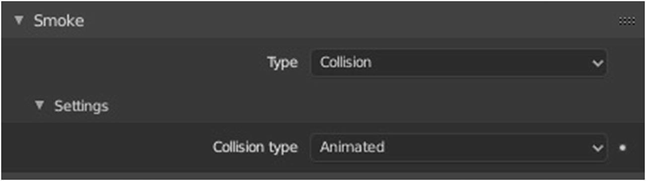
Smoke Simulation Physics ➤ Collision Type
Collision type of Smoke have a few settings. There are three types: Static, Rigid, and Animated.
Smoke ➤ Flow Type

Smoke Simulation Physics ➤Flow Type ➤ Fire +Smoke settings
Flow Source (Fire, Smoke, Fire+Smoke). Where you can change how smoke is emitted. There are two options: Mesh and Particle.
Surface (Fire, Smoke, Fire+Smoke). Maximum distance from mesh surface to emit smoke.
Volume (Fire, Smoke, Fire+Smoke). Factor for smoke emitted from inside the mesh volume.
Absolute Density (Fire, Smoke, Fire+Smoke). Only allow given density value in temperature density.
Density (Smoke, Fire+Smoke). Specifies the value for density.
Temperature Difference (Smoke, Fire+Smoke). Specifies the temperature difference to ambient temperature.
Smoke Color (Smoke, Fire+Smoke). Specifies the color of smoke.
Flame Rate (Fire, Fire+Smoke). Specifies the flame rate.
Sampling Subframes (Fire, Smoke, Fire+Smoke). Number of additional samples to take between frames to improve quality of fast moving flows.
Vertex Group (Fire, Outflow, Smoke, Fire+Smoke). The name of the vertex group that determines the surface emission rate.
Initial Velocity ➤ Source (Fire, Smoke, Fire+Smoke). Multiplier of source velocity passed to smoke.
Initial Velocity ➤ Normal (Fire, Smoke, Fire+Smoke). The amount of normal directional velocity.
Texture ➤ Texture (Fire, Outflow, Smoke, Fire+Smoke). Specifies texture that controls emission strength.
Texture ➤ Mapping (Fire, Outflow, Smoke, Fire+Smoke). Where you can choose texture mapping. There are two options: Generated and UV.
Texture ➤ Size (Fire, Outflow, Smoke, Fire+Smoke). Specifies the size of texture mapping.
Texture ➤ Offset (Fire, Outflow, Smoke, Fire+Smoke). Specifies the Z-offset of texture mapping.
Rigid Body Physics

The Rigid Body simulation simulates the motion of solid objects. It affects the position and orientation of objects and does not deform them.
Unlike the other simulations in Blender, the rigid body simulation works closer with the animation system. This means that rigid bodies can be used like regular objects and be part of parent-child relationships, animation constraints, and drivers.
Type. Role of object in Rigid Body Simulation. There are two types: Passive and Active.
Mass. Specifies how much the object weighs, irrespective of gravity. Only present in Active Type.
Dynamic. Rigid body actively participate to the simulation. Only present in Active type.
Animated. Allows Rigid Body to be controlled by the animation system.
Collisions ➤ Shape. Choose the collision shape of object in Rigid Body Simulation. There are seven options: Box, Sphere, Capsule, Cylinder, Cone, Convex Hull, and Mesh. By default, it is set to Convex Hull.
Collision Source ➤ Source. Set the source of mesh to create collision shape. This setting is only present when Shape is set to Convex Hull or Mesh.
Surface Response ➤ Friction. Resistance of object to movement.
Surface Response ➤ Bounciness. Tendency of object to bounce after colliding with another.
Sensitivity ➤ Collision Margin. Uses custom collision margin. This setting is not present when the Shape setting under Collision is set to Cone Shape.
Sensitivity ➤ Margin. Threshold of distance near surface where collisions are still considered.
Collections. Collision collections rigid body belongs to.
Rigid Body Constraints (Physics)

Rigid Body Constraints Physics
Type. Sets the type of rigid body constraint. There are eight types: Fixed, Point, Hinge, Slider, Piston, Generic, Generic Spring, and Motor. Fixed is the default type set in this setting.
Enabled. Enables the constraint.
Disable Collision. Disables collisions between constrained rigid bodies.
Breakable. Constraint can be broken if it receives an impulse above the threshold.
Threshold. Impulse threshold that must be reached for the constraint to break.
Angular ➤ X angle. Limits the rotation around the x axis. Only active when type is set to Generic.
Angular ➤ X Lower/Upper. Specifies the lower/upper limit of the x-axis rotation. Only active when type is set to Generic.
Angular ➤ Y angle. Limits the rotation around the y axis. Only active when type is set to Generic.
Angular ➤ Y Lower/Upper. Specifies the lower/upper limit of the y-axis rotation. Only active when type is set to Generic.
Angular ➤ Z angle. Limits the rotation around the z axis.
Angular ➤ Z Lower/Upper. Specifies the lower/upper limit of the z-axis rotation. Only active when type is set to Hinge, Piston or Generic.
Angular ➤ Target Velocity. Specifies target angular motor velocity. Only active when type is set to motor.
Angular ➤ Max Impulse. Specifies maximum angular motor impulse. Only active when type is set to motor.
Linear ➤ X Axis. Limit translation on the x axis. Only active when Type is set to Piston and Generic.
Linear ➤ X Lower/Upper. Specifies the lower/upper limit of the x-axis translation. Only active when Type is set to Piston and Generic.
Linear ➤ Y Axis. Limit translation on the y axis. Only active when Type is set to Generic.
Linear ➤ Y Lower/Upper. Specifies the lower/upper limit of the y-axis translation. Only active when Type is set to Generic.
Linear ➤ Z Axis. Limit translation on the z axis. Only active when Type is set to Generic.
Linear ➤ Z Lower/Upper. Specifies Lower/Upper limit of the z-axis translation. Only active when Type is set to Generic.
Linear ➤ Target Velocity. Specifies target linear motor velocity. Only active when type is set to motor.
Linear ➤ Max Impulse. Specifies maximum linear motor impulse. Only active when type is set to motor.
Objects ➤ First/Second. Specifies First/Second Rigid Body to be constrained.
Override ➤ Iterations. Specifies number of constraint solver iterations needs per simulation step.
To learn more about how to use Blender Physics, visit https://docs.blender.org/manual/en/latest/physics/index.html.
I’d like for you to read Blender Manual since most of the information came from it. For now, it isn’t fully updated. You can also learn a lot from Blender Stack Exchange and Blenderartist.org, where I also got some of the information. Communicating with other 3D artists and researching are also essential.