7

Basics of Classes and Objects

The point of computing is to process data. We often encapsulate the processing and the data into a single definition. We can organize objects into classes with a common collection of attributes to define their internal state and common behavior. Each instance of a class is a distinct object with unique internal state.

This concept of state and behavior applies particularly well to the way games work. When building something like an interactive game, the user's actions update the game state. Each of the player's possible actions is a method to change the state of the game. In many games this leads to a lot of animation to show the transition from state to state. In a single-player arcade-style game, the enemies or opponents will often be separate objects, each with an internal state that changes based on other enemy actions and the player's actions.

On the other hand, when we think of a casino game, such as Craps, there are only two game states, called "point off" and "point on." The transitions are shown to players by moving markers and chips around on a casino table. The game state changes based on rolls of the dice, irrespective of the player's betting actions.

The point of object-oriented design is to define current state with attributes of an object. The object is a member of a broader class of similar objects. The methods of each member of the class will lead to state changes on that object.

In this chapter, we will look at the following recipes:

• Using a class to encapsulate data and processing
• Essential type hints for class definitions
• Designing classes with lots of processing
• Using typing.NamedTuple for immutable objects
• Using dataclasses for mutable objects
• Using frozen dataclasses for immutable objects
• Optimizing small objects with __slots__
• Using more sophisticated collections
• Extending a built-in collection – a list that does statistics
• Using properties for lazy attributes
• Creating contexts and context managers
• Managing multiple contexts with multiple resources

The subject of object-oriented design is quite large. In this chapter, we'll cover some of the essentials. We'll start with some foundational concepts, such as how a class definition encapsulates state and processing details for all instances of a class.

Using a class to encapsulate data and processing

Class design is influenced by the SOLID design principles. The Single Responsibility and Interface Segregation principles offer helpful advice. Taken together, these principles advise us that a class should have methods narrowly focused on a single, well-defined responsibility.

Another way of considering a class is as a group of closely-related functions working with common data. We call these methods for working with the data. A class definition should contain the smallest collection of methods for working with the object's data.

We'd like to create class definitions based on a narrow allocation of responsibilities. How can we define responsibilities effectively? What's a good way to design a class?

Getting ready

Let's look at a simple, stateful object—a pair of dice. The context for this is an application that simulates a simple game like Craps. This simulation can help measure the house edge, showing exactly how much money we can lose playing Craps.

There's an important distinction between a class definition and the various instances of the class, called objects or instances of the class. Our focus is on writing class definitions that describe the objects' state and behavior. Our overall application works by creating instances of the classes. The behavior that emerges from the collaboration of the objects is the overall goal of the design process.

This idea is called emergent behavior. It is an essential ingredient in object-oriented programming. We don't enumerate every behavior of a program. Instead, we decompose the program into objects, with state and behavior captured in class definitions. The interactions among the objects lead to the observable behavior. Because the definition is not in a single block of code, the behavior emerges from the ways separate objects collaborate.

A software object can be viewed as analogous to a thing—a noun. The behaviors of the class can then be viewed as verbs. This identification of nouns and verbs gives us a hint as to how we can proceed to design classes to work effectively.

This leads us to several steps of preparation. We'll provide concrete examples of these steps using a pair of dice for game simulation. We proceed as follows:

1. Write down simple sentences that describe what an instance of the class does. We can call these the problem statements. It's essential to focus on single-verb sentences, with a focus on only the nouns and verbs. Here are some examples:
   • The game of Craps has two standard dice.
   • Each die has six faces, with point values from one to six.
   • Dice are rolled by a player. (Or, using active-voice verbs, "A player rolls the dice.")
   • The total of the dice changes the state of the Craps game. Those rules are separate from the dice.
   • If the two dice match, the number was rolled the hard way. If the two dice do not match, the roll was made the easy way. Some bets depend on this hard-easy distinction.
2. Identify all of the nouns in the sentences. In this example, the nouns include dice, faces, point values, and player. Nouns may identify different classes of objects. These are collaborators. Examples of collaborators include player and game. Nouns may also identify attributes of objects in questions. Examples include face and point value.
3. Identify all the verbs in the sentences. Verbs are generally methods of the class in question. In this example, verbs include roll and match. Sometimes, they are methods of other classes. One example is to change the state of a game, which applies to a Craps object more than the dice object.
4. Identify any adjectives. Adjectives are words or phrases that clarify a noun. In many cases, some adjectives will clearly be properties of an object. In other cases, the adjectives will describe relationships among objects. In our example, a phrase such as the total of the dice is an example of a prepositional phrase taking the role of an adjective. The the total of phrase modifies the noun the dice. The total is a property of the pair of dice.

This information is essential for defining the state and behavior of the objects. Having his background information will help us write the class definition.

How to do it...

Since the simulation we're writing involves random throws of dice, we'll depend on from random import randint to provide the useful randint() function. Given a low and a high value, this returns a random number between the two values; both end values are included in the domain of possible results:

1. Start writing the class with the class statement:

   class Dice: 
   

2. Initialize the object's attributes with an __init__() method. We'll model the internal state of the dice with a faces attribute. The self variable is required to be sure that we're referencing an attribute of a given instance of a class. Prior to the first roll of the dice, the faces don't really have a well-defined value, so we'll use the tuple (0, 0). We'll provide a type hint on each attribute to be sure it's used properly throughout the class definition:

       def __init__(self) -> None: 
           self.faces: Tuple[int, int] = (0, 0)
   

3. Define the object's methods based on the various verbs. When the player rolls the dice, a roll() method can set the values shown on the faces of the two dice. We implement this with a method to set the faces attribute of the self object:

       def roll(self) -> None: 
           self.faces = (randint(1,6), randint(1,6))
   

   This method mutates the internal state of the object. We've elected to not return a value. This makes our approach somewhat like the approach of Python's built-in collection classes where a method that mutates the object does not return a value.

4. After a player rolls the dice, a total() method helps compute the total of the dice. This can be used by a separate object to change the state of the game based on the current state of the dice:

       def total(self) -> int: 
           return sum(self.faces)
   

5. To resolve bets, two more methods can provide Boolean answers to the hard-way and easy-way questions:

       def hardway(self) -> bool: 
           return self.faces[0] == self.faces[1]
       def easyway(self) -> bool: 
           return self.faces[0] != self.faces[1]
   

It's rare for a casino game to have a rule that has a simple logical inverse. It's more common to have a rare third alternative that has a remarkably bad payoff rule. These two methods are a rare exception to the common pattern.

Here's an example of using this Dice class:

1. First, we'll seed the random number generator with a fixed value so that we can get a fixed sequence of results. This is a way of creating a unit test for this class:

   >>> import random
   >>> random.seed(1)
   

2. We'll create a Dice object, d1. We can then set its state with the roll() method. We'll then look at the total() method to see what was rolled. We'll examine the state by looking at the faces attribute:

   >>> from ch06_r01 import Dice
   >>> d1 = Dice()
   >>> d1.roll()
   >>> d1.total()
   7
   >>> d1.faces
   (6, 1)
   

3. We'll create a second Dice object, d2. We can then set its state with the roll() method. We'll look at the result of the total() method, as well as the hardway() method. We'll examine the state by looking at the faces attribute:

   >>> d2 = Dice()
   >>> d2.roll()
   >>> d2.total()
   7
   >>> d2.hardway()
   False
   >>> d2.faces
   (1, 6)
   

4. Since the two objects are independent instances of the Dice class, a change to d2 has no effect on d1.

How it works...

The core idea here is to use ordinary rules of grammar—nouns, verbs, and adjectives—as a way to identify basic features of a class. In our example, dice are real things. We try to avoid using abstract terms such as randomizers or event generators. It's easier to describe the tangible features of real things, and then define an implementation to match the tangible features.

The idea of rolling the dice is an example physical action that we can model with a method definition. This action of rolling the dice changes the state of the object. In rare cases—1 time in 36—the next state will happen to match the previous state.

Adjectives often hold the potential for confusion. The following are descriptions of the most common ways in which adjectives operate:

• Some adjectives, such as first, last, least, most, next, and previous, will have a simple interpretation. These can have a lazy implementation as a method, or an eager implementation as an attribute value.
• Some adjectives are a more complex phrase, such as the total of the dice. This is an adjective phrase built from a noun (total) and a preposition (of). This, too, can be seen as a method or an attribute.
• Some adjectives involve nouns that appear elsewhere in our software. We might have a phrase such as the state of the Craps game, where state of modifies another object, the Craps game. This is clearly only tangentially related to the dice themselves. This may reflect a relationship between dice and game.
• We might add a sentence to the problem statement such as the dice are part of the game. This can help clarify the presence of a relationship between game and dice. Prepositional phrases, such as are part of, can always be reversed to create the statement from the other object's point of view: for example, The game contains dice. This can help clarify the relationships among objects.

In Python, the attributes of an object are by default dynamic. We don't specify a fixed list of attributes. We can initialize some (or all) of the attributes in the __init__() method of a class definition. Since attributes aren't static, we have considerable flexibility in our design.

There's more...

Capturing the essential internal state and methods that cause state change is the first step in good class design. We can summarize some helpful design principles using the acronym SOLID :

• Single Responsibility Principle: A class should have one clearly defined responsibility.
• Open/Closed Principle: A class should be open to extension – generally via inheritance – but closed to modification. We should design our classes so that we don't need to tweak the code to add or change features.
• Liskov Substitution Principle: We need to design inheritance so that a subclass can be used in place of the superclass.
• Interface Segregation Principle: When writing a problem statement, we want to be sure that collaborating classes have as few dependencies as possible. In many cases, this principle will lead us to decompose large problems into many small class definitions.
• Dependency Inversion Principle: It's less than ideal for a class to depend directly on other classes. It's better if a class depends on an abstraction, and a concrete implementation class is substituted for the abstract class.

The goal is to create classes that have the necessary behavior and also adhere to the design principles so they can be extended and reused.

See also

• See the Using properties for lazy attributes recipe, where we'll look at the choice between an eager attribute and a lazy property.
• In Chapter 8, More Advanced Class Design, we'll look in more depth at class design techniques.
• See Chapter 11, Testing, for recipes on how to write appropriate unit tests for the class.

Essential type hints for class definitions

A class name is also a type hint, allowing a direct reference between a variable and the class that should define the objects associated with the variable. This relationship lets tools such as mypy reason about our programs to be sure that object references and method references appear to match the type hints in our code.

We'll use type hints in three common places in a class definition:

• In method definitions, we'll use type hints to annotate the parameters and the return type.
• In the __init__() method, we may need to provide hints for the instance variables that define the state of the object.
• Any attributes of the class overall. These are not common and type hints are rare here.

Getting ready

We're going to examine a class with a variety of type hints. In this example, our class will model a handful of dice. We'll allow rerolling selected dice, making the instance of the class stateful.

The collection of dice can be set by a first roll, where all the dice are rolled. The class allows subsequent rolls of a subset of dice. The number of rolls is counted, as well.

The type hints will reflect the nature of the collection of dice, the integer counts, a floating-point average value, and a string representation of the hand as a whole. This will show a number of type hints and how to write them.

How to do it…

1. This definition will involve random numbers as well as type hints for sets and lists. We import the random module. From the typing module, we'll import only the types we need, Set and List:

   import random
   from typing import Set, List
   

2. Define the class. This is a new type as well:

   class Dice:
   

3. It's rare for class-level variables to require a type hint. They're almost always created with assignment statements that make the type information clear to a person or a tool like mypy. In this case, we want all instances of our class of dice to share a common random number generator:

       RNG = random.Random()
   

4. The __init__() method creates the instance variables that define the state of the object. In this case, we'll save some configuration details, plus some internal state. The __init__() method also has the initialization parameters. Generally, we'll put the type hints on these parameters. Other internal state variables may require type hints to show what kinds of values will be assigned by other methods of the class. In this example, the faces attribute has no initial value; we state that when it is set, it will be a List[int] object:

       def __init__(self, n: int, sides: int = 6) -> None:
           self.n_dice = n
           self.sides = sides
           self.faces: List[int]
           self.roll_number = 0
   

5. Methods that compute new derived values can be annotated with their return type information. Here are three examples to return a string representation, compute the total, and also compute an average of the dice. These functions have return types of str, int, and float, as shown:

       def __str__(self) -> str:
           return ", ".join(
               f"{i}: {f}"
               for i, f in enumerate(self.faces)
           )
       def total(self) -> int:
           return sum(self.faces)
       def average(self) -> float:
           return sum(self.faces) / self.n_dice
   

6. For methods with parameters, we include type hints on the parameters as well as a return type. In this case, the methods that change the internal state also return values. The return value from both methods is a list of dice faces, described as List[int]. The parameter for the reroll() method is a set of dice to be rolled again, this is shown as a Set[int] requiring a set of integers. Python is a little more flexible than this, and we'll look at some alternatives:

   def first_roll(self) -> List[int]:
       self.roll_number = 0
       self.faces = [
           self.RNG.randint(1, self.sides)
           for _ in range(self.n_dice)
       ]
       return self.faces
   def reroll(self, positions: Set[int]) -> List[int]:
       self.roll_number += 1
       for p in positions:
           self.faces[p] = self.RNG.randint(1, self.sides)
       return self.faces
   

How it works…

The type hint information is used by programs such as mypy to be sure the instances of the class are used properly through the application.

If we try to write a function like the following:

def example_mypy_failure() -> None:
    d = Dice(2.5)
    d.first_roll()
    print(d)

This attempt to create an instance of the Dice() class using a float value for the n parameter represents a conflict with the type hints. The hint for the Dice class __init__() method claimed the argument value should be an integer. The mypy program reports the following:

Chapter_07/ch07_r02.py:49: error: Argument 1 to "Dice" has incompatible type "float"; expected "int"

If we try to execute this, it will raise a TypeError exception on using the d.first_roll() method. The exception is raised here because the body of the __init__() method works well with values of any type. The hints claim specific types are expected, but at runtime, any object can be provided. The hints are not checked during execution.

Similarly, when we use other methods, the mypy program checks to be sure our use of the method matches the expectations defined by the type hints. Here's another example:

r1: List[str] = d.first_roll()

This assignment statement has a type hint for the r1 variable that doesn't match the type hint for the return type from the first_roll() method. This conflict is found by mypy and reported as Incompatible types in assignment.

There's more…

One of the type hints in this example is too specific. The function for re-rolling the dice, reroll(), has a positions parameter. The positions parameter is used in a for statement, which means the object must be some kind of iterable object.

The mistake was providing a type hint, Set[int], which is only one of many kinds of iterable objects. We can generalize this definition by switching the type hint from the very specific Set[int] to the more general Iterable[int].

Relaxing the hint means that a set, list, or tuple object is a valid argument value for this parameter. The only other code change required is to add Iterable to the from typing import statement.

The for statement has a specific protocol for getting the iterator object from an iterable collection, assigning values to a variable, and executing the indented body. This protocol is defined by the Iterable type hint. There are many such protocol-based types, and they allow us to provide type hints that match Python's inherent flexibility with respect to type.

See also

• In Chapter 4, Built-In Data Structures Part 1: Lists and Sets, the recipes Writing list-related type hints, Writing set-related type hints, and Writing dictionary-related type hints address additional detailed type hinting.
• In Chapter 3, Function Definitions, in the recipe Function Parameters and Type Hints, a number of similar concepts are shown.

Designing classes with lots of processing

Some of the time, an object will contain all of the data that defines its internal state. There are cases, however, where a class doesn't hold the data, but instead is designed to consolidate processing for data held in separate containers.

Some prime examples of this design are statistical algorithms, which are often outside the data being analyzed. The data might be in a built-in list or Counter object; the processing defined in a class separate from the data container.

In Python, we have to make a design choice between a module and a class. A number of related operations can be implemented using a module with many functions. See Chapter 3, Function Definitions, for more information on this.

A class definition can be an alternative to a module with a number of functions. How can we design a class that makes use of Python's sophisticated built-in collections as separate objects?

Getting ready

In Chapter 4, Built-In Data Structures Part 1: Lists and Sets, specifically the Using set methods and operators recipe, we looked at a statistical test called the Coupon Collector's Test. The concept is that each time we perform some process, we save a coupon that describes some aspect or parameter for the process. The question is, how many times do I have to perform the process before I collect a complete set of coupons?

If we have customers assigned to different demographic groups based on their purchasing habits, we might ask how many online sales we have to make before we've seen someone from each of the groups. If the groups are all about the same size, we can predict the average number of customers we encounter before we get a complete set of coupons. If the groups are different sizes, it's a little more complex to compute the expected time before collecting a full set of coupons.

Let's say we've collected data using a Counter object. In this example, the customers fall into eight categories with approximately equal numbers.

The data looks like this:

Counter({15: 7, 17: 5, 20: 4, 16: 3, ... etc., 45: 1})

The keys (15, 17, 20, 16, and so on) are the number of customer visits needed to get a full set of coupons from all the demographic groups. We've run the experiment many times, and the value associated with this key is the number of experiment trials with the given number of visits. In the preceding data, 15 visits were required on seven different trials. 17 visits were required for five different trials. This has a long tail. For one of the experimental trials, there were 45 individual visits before a full set of eight coupons was collected.

We want to compute some statistics on this Counter. We have two general strategies for storing the data:

• Extend: We can extend the Counter class definition to add statistical processing. The complexity of this varies with the kind of processing that we want to introduce. We'll cover this in detail in the Extending a built-in collection – a list that does statistics recipe, as well as Chapter 8, More Advanced Class Design.
• Wrap: We can wrap the Counter object in another class that provides just the features we need. When we do this, though, we'll often have to expose some additional methods that are an important part of Python, but that don't matter much for our application. We'll look at this in Chapter 8, More Advanced Class Design.

There's a variation on the wrap strategy where we define a statistical computation class that contains a Counter object. This often leads to an elegant solution.

We have two ways to design this separate processing. These two design alternatives apply to all of the architectural choices for storing the data:

• Eager: This means that we'll compute the statistics as soon as possible. The values can then be attributes of the class. While this can improve performance, it also means that any change to the data collection will invalidate the eagerly computed values, leading to a need to recompute them to keep them consistent with the data. We have to examine the overall context to see if this can happen.
• Lazy: This means we won't compute anything until it's required via a method function or property. We'll look at this in the Using properties for lazy attributes recipe.

The essential math for both designs is the same. The only question is when the computation is done.

We compute the mean using a sum of the expected values. The expected value is the frequency of a value multiplied by the value. The mean, , is this:

Here, k is the key from the Counter, C, and f_k is the frequency value for the given key from the Counter. We weight each key with the number of times it was found in the Counter collection out of the total size of the collection, the sum of all the counts.

The standard deviation, , depends on the mean, . This also involves computing a sum of values, each of which is weighted by frequency. The following is the formula:

Here, k is the key from the Counter, C, and f_k is the frequency value for the given key from the Counter. The total number of items in the Counter is . This is the sum of the frequencies.

How to do it...

1. Import the collections module as well as the type hint for the collection that will be used:

   import collections
   from typing import Counter
   

2. Define the class with a descriptive name:

   class CounterStatistics:
   

3. Write the __init__() method to include the object where the data is located. In this case, the type hint is Counter[int] because the keys used in the collections.Counter object will be integers. The typing.Collection and counter.Collection names are similar. To avoid confusion, it's slightly easier if the names from the typing module are imported directly, and the related collection.Counter class uses the full name, qualified by module:

       def __init__(self, raw_counter: Counter[int]) -> None:
           self.raw_counter = raw_counter
   

4. Initialize any other local variables in the __init__() method that might be useful. Since we're going to calculate values eagerly, the most eager possible time is when the object is created. We'll write references to some yet to be defined functions:

           self.mean = self.compute_mean()
           self.stddev = self.compute_stddev()
   

5. Define the required methods for the various values. Here's the calculation of the mean:

       def compute_mean(self) -> float:
           total, count = 0.0, 0
           for value, frequency in self.raw_counter.items():
               total += value * frequency
               count += frequency
           return total / count
   

6. Here's how we can calculate the standard deviation:

       def compute_stddev(self) -> float:
           total, count = 0.0, 0
           for value, frequency in self.raw_counter.items():
               total += frequency * (value - self.mean) ** 2
               count += frequency
           return math.sqrt(total / (count - 1))
   

Note that this calculation requires that the mean is computed first and the self.mean instance variable has been created. Also, this uses math.sqrt(). Be sure to add the needed import math statement in the Python file.

Here's how we can create some sample data:

from Chapter_15.collector import (
    samples, arrival1, coupon_collector
)
import collections
ArrivalF = Callable[[int], Iterator[int]]
def raw_data(
    n: int = 8, limit: int = 1000, 
    arrival_function: ArrivalF = arrival1
) -> Counter[int]:
    data = samples(limit, arrival_function(n))
    wait_times = collections.Counter(coupon_collector(n, data))
    return wait_times

We've imported functions such as expected(), arrival1(), and coupon_collector() from the Chapter_15.collector module. We've also imported the standard library collections module.

The type definition for ArrivalF describes a function used to compute individual arrivals. For our simulation purposes, we've defined a number of these functions, each of which emits a sequence of customer coupons. When working with actual sales receipts, this can be replaced with a function that reads source datasets. All the functions have a common structure of accepting a domain size and emitting a sequence of values from the domain.

The raw_data() function will generate a number of customer visits. By default, it will be 1,000 visits. The domain will be eight different classes of customers; each class will have an equal number of members. We'll use the coupon_collector() function to step through the data, emitting the number of visits required to collect a full set of eight coupons.

This data is then used to assemble a collections.Counter object. This will have the number of customers required to get a full set of coupons. Each number of customers will also have a frequency showing how often that number of visits occurred. Because the key is the integer count of the number of visits, the type hint is Counter[int].

Here's how we can analyze the Counter object:

>>> import random
>>> from ch07_r03 import CounterStatistics
>>> random.seed(1)
>>> data = raw_data()
>>> stats = CounterStatistics(data)
>>> print("Mean: {0:.2f}".format(stats.mean))
Mean: 20.81
>>> print("Standard Deviation: {0:.3f}".format(stats.stddev))
Standard Deviation: 7.025

First, we imported the random module so that we could pick a known seed value. This makes it easier to test and demonstrate an application because the random numbers are consistent. We also imported the CounterStatistics class from the ch07_r03 module.

Once we have all of the items defined, we can force the seed to a known value, and generate the coupon collector test results. The raw_data() function will emit a Counter object, which we called data.

We'll use the Counter object to create an instance of the CounterStatistics class. We'll assign this to the stats variable. Creating this instance will also compute some summary statistics. These values are available as the stats.mean attribute and the stats.stddev attribute.

For a set of eight coupons, the theoretical average is 21.7 visits to collect all coupons. It looks like the results from raw_data() show behavior that matches the expectation of random visits. This is sometimes called the null hypothesis—the data is random.

How it works...

This class encapsulates two complex algorithms, but doesn't include any of the data for those algorithms. The data is kept separately, in a Counter object. We wrote a high-level specification for the processing and placed it in the __init__() method. Then we wrote methods to implement the processing steps that were specified. We can set as many attributes as are needed, making this a very flexible approach.

The advantage of this design is that the attribute values can be used repeatedly. The cost of computation for the mean and standard deviation is paid once; each time an attribute value is used, no further calculating is required.

The disadvantage of this design is changes to the state of the underlying Counter object will render the CounterStatistics object's state obsolete and incorrect. If, for example, we added a few hundred more trial runs, the mean and standard deviation would need to be recomputed. A design that eagerly computes values is appropriate when the underlying Counter isn't going to change. An eager design works well for batches of data with few changes.

There's more...

If we need to have stateful, mutable objects, we can add update methods that can change the Counter object's internal state. For example, we can introduce a method to add another value by delegating the work to the associated Counter. This switches the design pattern from a simple connection between computation and collection to a proper wrapper around the collection.

The method might look like this:

    def add(self, value: int) -> None:
        self.raw_counter[value] += 1
        self.mean = self.compute_mean()
        self.stddev = self.compute_stddev()

First, we updated the state of the Counter. Then, we recomputed all of the derived values. This kind of processing might create tremendous computation overheads. There needs to be a compelling reason to recompute the mean and standard deviation after every value is changed.

There are considerably more efficient solutions. For example, if we save two intermediate sums and an intermediate count, we can update the sums and counts and compute the mean and standard deviation more efficiently.

For this, we might have an __init__() method that looks like this:

def __init__(self, counter: Counter = None) -> None:
    if counter is not None:
        self.raw_counter = counter
        self.count = sum(
            self.raw_counter[k] for k in self.raw_counter)
        self.sum = sum(
            self.raw_counter[k] * k for k in self.raw_counter)
        self.sum2 = sum(
            self.raw_counter[k] * k ** 2
                for k in self.raw_counter)
        self.mean: Optional[float] = self.sum / self.count
        self.stddev: Optional[float] = math.sqrt(
            (self.sum2 - self.sum ** 2 / self.count)
            / (self.count - 1)
        )
    else:
        self.raw_counter = collections.Counter()
        self.count = 0
        self.sum = 0
        self.sum2 = 0
        self.mean = None
        self.stddev = None

We've written this method to work either with a Counter object or without an initialized Counter instance. If no data is provided, it will start with an empty collection, and zero values for the count and the various sums. When the count is zero, the mean and standard deviation have no meaningful value, so None is provided.

If a Counter is provided, then count, sum, and the sum of squares are computed. These can be incrementally adjusted easily, quickly recomputing the mean and standard deviation.

When a single new value needs to be added to the collection, the following method will incrementally recompute the derived values:

def add(self, value: int) -> None:
    self.raw_counter[value] += 1
    self.count += 1
    self.sum += value
   self.sum2 += value ** 2
    self.mean = self.sum / self.count
    if self.count > 1:
        self.stddev = math.sqrt(
            (self.sum2 - self.sum ** 2 / self.count)
            / (self.count - 1)
        )

Updating the Counter object, the count, the sum, and the sum of squares is clearly necessary to be sure that the count, sum, and sum of squares values match the self.raw_counter collection at all times. Since we know the count must be at least 1, the mean is easy to compute. The standard deviation requires at least two values, and is computed from the sum and the sum of squares.

Here's the formula for this variation on standard deviation:

This involves computing two sums. One sum involves the frequency times the value squared. The other sum involves the frequency and the value, with the overall sum being squared. We've used C to represent the total number of values; this is the sum of the frequencies.

See also

• In the Extending a built-in collection – a list that does statistics recipe, we'll look at a different design approach where these functions are used to extend a class definition.
• We'll look at a different approach in the Using properties for lazy attributes recipe. This alternative recipe will use properties and compute the attributes as needed.
• In the Designing classes with little unique processing recipe, we'll look at a class with no real processing. It acts as a polar opposite of this class.

Using typing.NamedTuple for immutable objects

In some cases, an object is a container of rather complex data, but doesn't really do very much processing on that data. Indeed, in many cases, we'll define a class that doesn't require any unique method functions. These classes are relatively passive containers of data items, without a lot of processing.

In many cases, Python's built-in container classes – list, set, or dict – can cover the use cases. The small problem is that the syntax for a dictionary or a list isn't quite as elegant as the syntax for attributes of an object.

How can we create a class that allows us to use object.attribute syntax instead of object['attribute']?

Getting ready

There are two cases for any kind of class design:

• Is it stateless (immutable)? Does it embody attributes with values that never change? This is a good example of a NamedTuple.
• Is it stateful (mutable)? Will there be state changes for one or more attributes? This is the default for Python class definitions. An ordinary class is stateful. We can simplify creating stateful objects using the recipe Using dataclasses for mutable objects.

We'll define a class to describe simple playing cards that have a rank and a suit. Since a card's rank and suit don't change, we'll create a small stateless class for this. typing.NamedTuple serves as a handy base class for this class definition.

How to do it...

1. We'll define stateless objects as a subclass of typing.NamedTuple:

   from typing import NamedTuple
   

2. Define the class name as an extension to NamedTuple. Include the attributes with their individual type hints:

   class Card(NamedTuple):
       rank: int
       suit: str
   

Here's how we can use this class definition to create Card objects:

>>> eight_hearts = Card(rank=8, suit='N{White Heart Suit}')
>>> eight_hearts
Card(rank=8, suit='')
>>> eight_hearts.rank
8
>> eight_hearts.suit
''
>>> eight_hearts[0]
8

We've created a new class, named Card, which has two attribute names: rank and suit. After defining the class, we can create an instance of the class. We built a single card object, eight_hearts, with a rank of eight and a suit of .

We can refer to attributes of this object with their name or their position within the tuple. When we use eight_hearts.rank or eight_hearts[0], we'll see the rank attribute because it's defined first in the sequence of attribute names.

This kind of object is immutable. Here's an example of attempting to change the instance attributes:

>>> eight_hearts.suit = 'N{Black Spade Suit}'
Traceback (most recent call last):
  File "/Users/slott/miniconda3/envs/cookbook/lib/python3.8/doctest.py", line 1328, in __run
    compileflags, 1), test.globs)
  File "<doctest examples.txt[30]>", line 1, in <module>
    eight_hearts.suit = 'N{Black Spade Suit}'
AttributeError: can't set attribute

We attempted to change the suit attribute of the eight_hearts object. This raised an AttributeError exception showing that instances of NamedTuple are immutable.

How it works...

The typing.NamedTuple class lets us define a new subclass that has a well-defined list of attributes. A number of methods are created automatically to provide a minimal level of Python behavior. We can see an instance will display a readable text representation showing the values of the various attributes.

In the case of a NamedTuple subclass, the behavior is based on the way a built-in tuple instance works. The order of the attributes defines the comparison between tuples. Our definition of Card, for example, lists the rank attribute first. This means that we can easily sort cards by rank. For two cards of equal rank, the suits will be sorted into order. Because a NamedTuple is also a tuple, it works well as a member of a set or a key for a dictionary.

The two attributes, rank and suit in this example, are named as part of the class definition, but are implemented as instance variables. A variation on the tuple's __new__() method is created for us. This method has two parameters matching the instance variable names. This automatically created method will assign the instance variables automatically when the object is created.

There's more...

We can add methods to this class definition. For example, if each card has a number of points, we might want to extend the class to look like this example:

class CardPoints(NamedTuple):
    rank: int
    suit: str
    def points(self) -> int:
        if 1 <= self.rank < 10:
            return self.rank
        else:
            return 10

We've written a CardsPoint class with a points() method that returns the points assigned to each rank. This point rule applies to games like Cribbage, not to games like Blackjack.

Because this is a tuple, the methods cannot add new attributes or change the attributes. In some cases, we build complex tuples built from other tuples.

See also

• In the Designing classes with lots of processing recipe, we looked at a class that is entirely processing and almost no data. It acts as the polar opposite of this class.

Using dataclasses for mutable objects

There are two cases for any kind of class design:

• Is it stateless (immutable)? Does it embody attributes with values that never change? If so, see the Using typing.NamedTuple for immutable objects recipe for a way to build class definitions for stateless objects.
• Is it stateful (mutable)? Will there be state changes for one or more attributes? In this case, we can either build a class from the ground up, or we can leverage the @dataclass decorator to create a class definition from a few attributes and type hints.

Getting ready

We'll look closely at a stateful object that holds a hand of cards. Cards can be inserted into a hand and removed from a hand. In a game like Cribbage, the hand has a number of state changes. Initially, six cards are dealt to both players. The players will each place a pair of cards in a special pile, called the crib. The remaining four cards are played alternately to create scoring opportunities. After each hand's scoring combinations are totalled, the dealer will count the additional scoring combinations in the crib.

We'll look at a simple collection to hold the cards and discard two that form the crib.

How to do it…

1. To define data classes, we'll import the dataclass decorator:

   from dataclasses import dataclass
   from typing import List
   

2. Define the new class as a dataclass:

   @dataclass
   class CribbageHand:
   

3. Define the various attributes with appropriate type hints. For this example, we'll expect a player to have a collection of cards represented by List[CardPoints]. Because each card is unique, we could also use a Set[CardPoints] type hint:

       cards: List[CardPoints]
   

4. Define any methods that change the state of the object:

       def to_crib(self, card1, card2):
           self.cards.remove(card1)
           self.cards.remove(card2)
   

Here's the complete class definition, properly indented:

@dataclass
class CribbageHand:
    cards: List[CardPoints]
    def to_crib(self, card1, card2):
        self.cards.remove(card1)
        self.cards.remove(card2)

This definition provides a single instance variable, self.cards, that can be used by any method that is written. Because we provided a type hint, the mypy program can check the class to be sure that it is being used properly.

Here's how it looks when we create an instance of this CribbageHand class:

>>> cards = [
... CardPoints(rank=3, suit=''), 
... CardPoints(rank=6, suit=''), 
.. CardPoints(rank=7, suit=''), 
... CardPoints(rank=1, suit=''), 
... CardPoints(rank=6, suit=''), 
... CardPoints(rank=10, suit='')]
>>> ch1 = CribbageHand(cards)
>>> ch1
CribbageHand(cards=[CardPoints(rank=3, suit=''), CardPoints(rank=6, suit=''), CardPoints(rank=7, suit=''), CardPoints(rank=1, suit=''), CardPoints(rank=6, suit=''), CardPoints(rank=10, suit='')])
>>> [c.points() for c in ch1.cards]
[3, 6, 7, 1, 6, 10]

We've created six individual CardPoints objects. This collection is used to initialize the CribbageHand object with six cards. In a more elaborate game, we might define a deck of cards and select from the deck.

The @dataclass decorator built a __repr__() method that returns a useful display string for the CribbageHand object. It shows the value of the card's instance variable. Because it's a display of six CardPoints objects, the text is long and sprawls over many lines. While the display may not be the prettiest, we wrote none of the code, making it very easy to use as a starting point for further development.

We built a small list comprehension showing the point values of each CardPoints object in the CribbageHand instance, ch1. A person uses this information (along with other details) to decide which cards to contribute to the dealer's crib.

In this case, the player decided to lay away the 3 and A cards for the crib:

>>> ch1.to_crib(CardPoints(rank=3, suit=''), CardPoints(rank=1, suit=''))
>>> ch1
CribbageHand(cards=[CardPoints(rank=6, suit=''), CardPoints(rank=7, suit=''), CardPoints(rank=6, suit=''), CardPoints(rank=10, suit='')])
>>> [c.points() for c in ch1.cards]
[6, 7, 6, 10]

After the to_crib() method removed two cards from the hand, the remaining four cards were displayed. Another list comprehension was created with the point values of the remaining four cards.

How it works…

The @dataclass decorator helps us define a class with several useful methods as well as a list of attributes drawn from the named variables and their type hints. We can see that an instance displays a readable text representation showing the values of the various attributes.

The attributes are named as part of the class definition, but are actually implemented as instance variables. In this example, there's only one attribute, cards. A very sophisticated __init__() method is created for us. In this example, it will have a parameter that matches the name of each instance variable and will assign a matching instance variable for us.

The @dataclass decorator has a number of options to help us choose what features we want in the class. Here are the options we can select from and the default settings:

• init=True: By default, an __init__() method will be created with parameters to match the instance variables. If we use @dataclass(init=False), we'll have to write our own __init__() method.
• repr=True: By default, a __repr__() method will be created to return a string showing the state of the object.
• eq=True: By default the __eq__() and __ne__() methods are provided. These will compare all of the instance variables. In the event this isn't appropriate, we can use @dataclass(eq=False) to turn this feature off. In some cases, equality doesn't apply, and the methods aren't needed. In other cases, the generated methods aren't appropriate for the class, and more specialized methods need to be written.
• order=False: The __lt__(), __le__(), __gt__(), and __ge__() methods are not created automatically. If these are built automatically, they will use all of the dataclass instance variables, which isn't always desirable.
• unsafe_hash=False: Normally, mutable objects do not have hash values, and cannot be used as keys for dictionaries or elements of a set. It's possible to have a __hash__() function added automatically, but this is rarely a sensible choice for mutable objects.
• frozen=False: This creates an immutable object. Using @dataclass(frozen=True) overlaps with typing.NamedTuple in many ways.

Because this code is written for us, it lets us focus on the attributes of the class definition. We can write the methods that are truly distinctive and avoid writing "boilerplate" methods that have obvious definitions.

There's more…

Building a deck of cards is an example of a dataclass without an initialization. A single deck of cards uses an __init__() method without any parameters, it creates a collection of 52 Card objects.

Many @dataclass definitions provide class-level names that are used to define the instance variables and the initialization method, __init__(). In this case, we want a class-level variable with a list of suit strings. This is done with the ClassVar type hint. The ClassVar type's parameters define the class-level variable's type. In this case, it's a tuple of strings:

from typing import List, ClassVar, Tuple
@dataclass(init=False)
class Deck:
    suits: ClassVar[Tuple[str, ...]] = (
        'N{Black Club Suit}', 'N{White Diamond Suit}',
        'N{White Heart Suit}', 'N{Black Spade Suit}'
    )
    cards: List[CardPoints]
    def __init__(self) -> None:
        self.cards = [
            CardPoints(rank=r, suit=s)
                for r in range(1, 14)
                    for s in self.suits
        ]
        random.shuffle(self.cards)

This example class definition provides a class-level variable, suits, which is shared by all instances of the Deck class. This variable is a tuple of the characters used to define the suits.

The cards variable has a hint claiming it will have the List[CardPoints] type. This information is used by the mypy program to confirm that the body of the __init__() method performs the proper initialization of this attribute. It also confirms this attribute is used appropriately by other classes.

The __init__() method creates the value of the self.cards variable. A list comprehension is used to create all combinations of 13 ranks and 4 suits. Once the list has been built, the random.shuffle() method puts the cards into a random order.

See also

• See the Using typing.NamedTuple for immutable objects recipe for a way to build class definitions for stateless objects.
• The Using a class to encapsulate data and processing recipe covers techniques for building a class without the additional methods created by the @dataclass decorator.

Using frozen dataclasses for immutable objects

In the Using typing.NamedTuple for immutable objects recipe, we saw how to define a class that has a fixed set of attributes. The attributes can be checked by the mypy program to ensure that they're being used properly. In some cases, we might want to make use of the slightly more flexible dataclass to create an immutable object.

One potential reason for using a dataclass is because it can have more complex field definitions than a NamedTuple subclass. Another potential reason is the ability to customize initialization and the hashing function that is created. Because a typing.NamedTuple is essentially a tuple, there's limited ability to fine-tune the behavior of the instances in this class.

Getting ready

We'll revisit the idea of defining simple playing cards with rank and suit. The rank can be modeled by an integer between 1 (ace) and 13 (king.) The suit can be modeled by a single Unicode character from the set {'', '', '', ''}. Since a card's rank and suit don't change, we'll create a small, frozen dataclass for this.

How to do it…

1. From the dataclasses module, import the dataclass decorator:

   from dataclasses import dataclass
   

2. Start the class definition with the @dataclass decorator, using the frozen=True option to ensure that the objects are immutable. We've also included order=True so that the comparison operators are defined, allowing instances of this class to be sorted into order:

   @dataclass(frozen=True, order=True)
   class Card:
   

3. Provide the attribute names and type hints for the attributes of each instance of this class:

       rank: int
       suit: str
   

We can use these objects in code like the following:

>>> eight_hearts = Card(rank=8, suit='N{White Heart Suit}')
>>> eight_hearts
Card(rank=8, suit='')
>>> eight_hearts.rank
8
>>> eight_hearts.suit
''

We've created an instance of the Card class with a specific value for the rank and suit attributes. Because the object is immutable, any attempt to change the state will result in an exception that looks like the following example:

>>> eight_hearts.suit = 'N{Black Spade Suit}'
Traceback (most recent call last):
  File "/Users/slott/miniconda3/envs/cookbook/lib/python3.8/doctest.py", line 1328, in __run
    compileflags, 1), test.globs)
  File "<doctest examples.txt[30]>", line 1, in <module>
    eight_hearts.suit = 'N{Black Spade Suit}'
dataclasses.FrozenInstanceError: cannot assign to field 'suit'

This shows an attempt to change an attribute of a frozen dataclass instance. The dataclasses.FrozenInstanceError exception is raised to signal that this kind of operation is not permitted.

How it works…

This @dataclass decorator adds a number of built-in methods to a class definition. As we noted in the Using dataclasses for mutable objects recipe, there are a number of features that can be enabled or disabled. Each feature may have one or several individual methods.

The type hints are incorporated into all of the generated methods. This assures consistency that can be checked by the mypy program.

There's more…

The dataclass initialization is quite sophisticated. We'll look at one feature that's sometimes handy for defining optional attributes.

Consider a class that can hold a hand of cards. While the common use case provides a set of cards to initialize the hand, we can also have hands that might be built incrementally, starting with an empty collection and adding cards during the game.

We can define this kind of optional attribute using the field() function from the dataclasses module. The field() function lets us provide a function to build default values, called default_factory. We'd use it as shown in the following example:

from dataclasses import field
from typing import List
@dataclass(frozen=True, order=True)
class Hand:
    cards: List[CardPoints] = field(default_factory=list)

The Hand dataclass has a single attribute, cards, which is a list of CardPoints objects. The field() function provides a default factory: in the event no initial value is provided, the list() function will be executed to create a new, empty list.

We can create two kinds of hands with this dataclass. Here's the conventional example, where we deal six cards:

>>> cards = [
... CardPoints(rank=3, suit=''), 
... CardPoints(rank=6, suit=''), 
... CardPoints(rank=7, suit=''),
... CardPoints(rank=1, suit=''), 
... CardPoints(rank=6, suit=''),
... CardPoints(rank=10, suit='')]
>>> 
>>> h = Hand(cards)

The Hands() type expects a single attribute, matching the definition of the attributes in the class. This is optional, and we can build an empty hand as shown in this example:

>>> crib = Hand()
>>> d3 = CardPoints(rank=3, suit='')
>>> h.cards.remove(d3)
>>> crib.cards.append(d3)

In this example, we've created a Hand() instance with no argument values. Because the cards attribute was defined with a field that provided a default_factory, the list() function will be used to create an empty list for the cards attribute.

See also

• The Using dataclasses for mutable objects recipe covers some additional topics on using dataclasses to avoid some of the complexities of writing class definitions.

Optimizing small objects with __slots__

The general case for an object allows a dynamic collection of attributes. There's a special case for an immutable object with a fixed collection of attributes based on the tuple class. We looked at both of these in the Designing classes with little unique processing recipe.

There's a middle ground. We can also define an object with a fixed number of attributes, but the values of the attributes can be changed. By changing the class from an unlimited collection of attributes to a fixed set of attributes, it turns out that we can also save memory and processing time.

How can we create optimized classes with a fixed set of attributes?

Getting ready

Let's look at the idea of a hand of playing cards in the casino game of Blackjack. There are two parts to a hand:

• The bet
• The cards

Both have dynamic values. Generally, each hand starts with a bet and an empty collection of cards. The dealer then deals two initial cards to the hand. It's common to get more cards. It's also possible to raise the bet via a double-down play.

Generally, Python allows adding attributes to an object. This can be undesirable, particularly when working with a large number of objects. The flexibility of using a dictionary has a high cost in memory use. Using specific __slots__ names limits the class to precisely the bet and the cards attributes, saving memory.

How to do it...

We'll leverage the __slots__ special name when creating the class:

1. Define the class with a descriptive name:

     class Hand: 
   

2. Define the list of attribute names. This identifies the only two attributes that are allowed for instances of this class. Any attempt to add another attribute will raise an AttributeError exception:

       __slots__ = ('cards', 'bet') 
   

3. Add an initialization method. In this example, we've allowed three different kinds of initial values for the cards. The type hint, Union["Hand", List[Card], None], permits a Hand instance, a List[Card] instance, or nothing at all. For more information on this, see the Designing functions with optional parameters recipe in Chapter 3, Function Definitions. Because the __slot__ names don't have type hints, we need to provide them in the __init__() method:

   def __init__(
           self,
           bet: int,
           hand: Union["Hand", List[Card], None] = None
   ) -> None:
       self.cards: List[Card] = (
           [] if hand is None
               else hand.cards if isinstance(hand, Hand)
                   else hand
       )
       self.bet: int = bet
   

4. Add a method to update the collection. We've called it deal because it's used to deal a new card to the hand:

       def deal(self, card: Card) -> None:
           self.cards.append(card)
   

5. Add a __repr__() method so that it can be printed easily:

   def __repr__(self) -> str:
       return (
           f"{self.__class__.__name__}("
           f"bet={self.bet}, hand={self.cards})"
       )
   

Here's how we can use this class to build a hand of cards. We'll need the definition of the Card class based on the example in the Designing classes with little unique processing recipe:

>>> from Chapter_07.ch07_r07 import Card, Hand
>>> h1 = Hand(2)
>>> h1.deal(Card(rank=4, suit=''))
>>> h1.deal(Card(rank=8, suit=''))
>>> h1
Hand(bet=2, hand=[Card(rank=4, suit=''), Card(rank=8, suit='')])

We've imported the Card and Hand class definitions. We built an instance of a Hand, h1, with a bet of 2. We then added two cards to the hand via the deal() method of the Hand class. This shows how the h1.hand value can be mutated.

This example also displays the instance of h1 to show the bet and the sequence of cards. The __repr__() method produces output that's in Python syntax.

We can replace the h1.bet value when the player doubles down (yes, this is a crazy thing to do when showing 12):

>>> h1.bet *= 2
>>> h1
Hand(bet=4, hand=[Card(rank=4, suit=''), Card(rank=8, suit='')])

When we displayed the Hand object, h1, it showed that the bet attribute was changed.

A better design than changing the bet attribute value is to introduce a double_down() method that makes appropriate changes to the Hand object.

Here's what happens if we try to create a new attribute:

>>> h1.some_other_attribute = True  
Traceback (most recent call last):
  File "/Users/slott/miniconda3/envs/cookbook/lib/python3.8/doctest.py", line 1336, in __run
    exec(compile(example.source, filename, "single",
  File "<doctest examples.txt[34]>", line 1, in <module>
    h1.some_other_attribute = True  
AttributeError: 'Hand' object has no attribute 'some_other_attribute' 

We attempted to create an attribute named some_other_attribute on the Hand object, h1. This raised an AttributeError exception. Using __slots__ means that new attributes cannot be added to the object.

How it works...

When we create an object instance, the steps in the process are defined in part by the object's class and the built-in type() function. Implicitly, a class is assigned a special __new__() method that handles the internal house-keeping required to create a new, empty object. After this, the __init__() method creates and initializes the attributes.

Python has three essential paths for creating instances of a class:

• The default behavior, defined by a built-in object and type(): This is used when we define a class with or without the @dataclass decorator. Each instance contains a __dict__ attribute that is used to hold all other attributes. Because the object's attributes are kept in a dictionary, we can add, change, and delete attributes freely. This flexibility requires the use of a relatively large amount of memory for the dictionary object inside each instance.
• The __slots__ behavior: This avoids creating the __dict__ attribute. Because the object has only the attributes named in the __slots__ sequence, we can't add or delete attributes. We can change the values of the defined attributes. This lack of flexibility means that less memory is used for each object.
• The subclass of tuple behavior: These are immutable objects. An easy way to create these classes is with typing.NamedTuple as a parent class. Once built, the instances are immutable and cannot be changed.

A large application might be constrained by the amount of memory used, and switching just the class with the largest number of instances to __slots__ can lead to a dramatic improvement in performance.

There's more...

It's possible to tailor the way the __new__() method works to replace the default __dict__ attribute with a different kind of dictionary. This is an advanced technique because it exposes the inner workings of classes and objects.

Python relies on a metaclass to create instances of a class. The default metaclass is the type class. The idea is that the metaclass provides a few pieces of functionality that are used to create the object. Once the empty object has been created, then the class's __init__() method will initialize the empty object.

Generally, a metaclass will provide a definition of __new__(), and perhaps __prepare__(), if there's a need to customize the namespace object. There's a widely used example in the Python Language Reference document that tweaks the namespace used to create a class.

For more details, see https://docs.python.org/3/reference/datamodel.html#metaclass-example.

See also

• The more common cases of an immutable object or a completely flexible object are covered in the Designing classes with little unique processing recipe.

Using more sophisticated collections

Python has a wide variety of built-in collections. In Chapter 4, Built-In Data Structures Part 1: Lists and Sets, we looked at them closely. In the Choosing a data structure recipe, we provided a kind of decision tree to help locate the appropriate data structure from the available choices.

When we consider built-ins and other data structures in the standard library, we have more choices, and more decisions to make. How can we choose the right data structure for our problem?

Getting ready

Before we put data into a collection, we'll need to consider how we'll gather the data, and what we'll do with the collection once we have it. The big question is always how we'll identify a particular item within the collection. We'll look at a few key questions that we need to answer to help select a proper collection for our needs.

Here's an overview of some of the alternative collections. The collections module contains a number of variations on the built-in collections. These include the following:

• deque: A double-ended queue. It's a mutable sequence with optimizations for pushing and popping from each end. Note that the class name starts with a lowercase letter; this is atypical for Python.
• defaultdict: A mapping that can provide a default value for a missing key. Note that the class name starts with a lowercase letter; this is atypical for Python.
• Counter: A mapping that is designed to count the number of occurrences of distinct keys. This is sometimes called a multiset or a bag.
• OrderedDict: A mapping that retains the order in which keys where created.
• ChainMap: A mapping that combines several dictionaries into a single mapping.

The heapq module includes a priority queue implementation. This is a specialized library that leverages the built-in list sequence to maintain items in a sorted order.

The bisect module includes methods for searching a sorted list. This creates some overlap between the dictionary features and the list features.

How to do it...

There are a number of questions we need to answer to decide if we need a library data collection instead of one of the built-in collections:

1. Is the structure a buffer between the producer and the consumer? Does some part of the algorithm produce data items and another part consume the data items?
   • A queue is used for First-In-First-Out (FIFO) processing. Items are inserted at one end and consumed from the other end. We can use list.append() and list.pop(0) to simulate this, though collections.deque will be more efficient; we can use deque.append() and deque.popleft().
   • A stack is used for Last-In-First-Out (LIFO) processing. Items are inserted and consumed from the same end. We can use list.append() and list.pop() to simulate this, though collections.deque will be more efficient; we can use deque.append() and deque.pop().
   • A priority queue (or heap queue) keeps the queue sorted in some order, distinct from the arrival order. We can try to simulate this by using the list.append(), list.sort(key=lambda x:x.priority), and list.pop(-1) operations to keep items in order. Performing a sort after each insert can make it inefficient. Folding an item into a previously sorted list doesn't necessarily touch all items. Using the heapq module can be more efficient. The heapq module has functions for creating and updating heaps.
2. How do we want to deal with missing keys from a dictionary?
   • Raise an exception. This is the way the built-in dict class works.
   • Create a default item. This is how collections.defaultdict works. We must provide a function that returns the default value. Common examples include defaultdict(int) and defaultdict(float) to use a default value of zero. We can also use defauldict(list) and defauldict(set) to create dictionary-of-list or dictionary-of-set structures.
   • The defaultdict(int) used to count items is so common that the collections.Counter class does exactly this.
3. How do we want to handle the order of keys in a dictionary? Generally, Python newer than version 3.6 keeps the keys in insertion order. If we want a different order, we'll have to sort them manually. See the Controlling the order of dict keys recipe for more details.
4. How will we build the dictionary?
   • We have a simple algorithm to create items. In this case, a built-in dict object may be sufficient.
   • We have multiple dictionaries that will need to be merged. This can happen when reading configuration files. We might have an individual configuration, a system-wide configuration, and a default application configuration that all need to be merged into a single dictionary using a ChainMap collection.

How it works...

There are two principle resource constraints on data processing:

• Storage
• Time

All of our programming must respect these constraints. In most cases, the two are in opposition: anything we do to reduce storage use tends to increase processing time, and anything we do to reduce processing time increases storage use. Algorithm and data structure design seeks to find an optimal balance among the constraints.

The time aspect is formalized via a complexity metric. There are several ways to describe the complexity of an algorithm:

• Complexity happens in constant time; the complexity doesn't change with the volume of data. For some collections, the actual overall long-term average is nearly with minor exceptions. List append operations are an example: they're all about the same complexity. Once in a while, though, a behind-the-scenes memory management operation will add some time.
• Complexity described as happens in linear time. The cost grows as the volume of data, n, grows. Finding an item in a list has this complexity. Finding an item in a dictionary is closer to because it's (nearly) the same low complexity, no matter how large the dictionary is.
• A complexity described as grows more quickly than the volume of data. Often the base two logarithm is used because each step in an algorithm considers only half the data. The bisect module includes search algorithms that have this complexity.
• There are even worse cases. Some algorithms have a complexity of , , or even . We'd like to avoid these kinds of very expensive algorithms through clever design and good choice of data structure. These can be deceptive in practice. We may be able to work out an algorithm where n is 3 or 4 because there are only 8 or 16 combinations, and the processing seems fast. If real data involves 70 items, the number of combinations has 22 digits.

The various data structures reflect unique time and storage trade-offs.

There's more...

As a concrete and extreme example, let's look at searching a web log file for a particular sequence of events. We have two overall design strategies:

• Read all of the events into a list structure with something like file.read().splitlines(). We can then use a for statement to iterate through the list looking for the combination of events. While the initial read may take some time, the search will be very fast because the log is all in memory.
• Read and process each individual event from a log file. If the event is part of the pattern, save just this event. We might use a defaultdict with the IP address as the key and a list of events as the value. This will take longer to read the logs, but the resulting structure in memory will be much smaller.

The first algorithm, reading everything into memory, is often wildly impractical. On a large web server, the logs might involve hundreds of gigabytes, or perhaps even terabytes, of data. Logs can easily be too large to fit into any computer's memory.

The second approach has a number of alternative implementations:

• Single process: The general approach to most of the Python recipes here assumes that we're creating an application that runs as a single process.
• Multiple processes: We might expand the row-by-row search into a multi-processing application using the multiprocessing or concurrent.futures package. These packages let us create a collection of worker processes, each of which can process a subset of the available data and return the results to a consumer that combines the results. On a modern multiprocessor, multi-core computer, this can be a very effective use of resources.
• Multiple hosts: The extreme case requires multiple servers, each of which handles a subset of the data. This requires more elaborate coordination among the hosts to share result sets. Generally, it can work out well to use a framework such as Dask or Spark for this kind of processing. While the multiprocessing module is quite sophisticated, tools like Dask are even more suitable for large-scale computation.

We'll often decompose a large search into map and reduce processing. The map phase applies some processing or filtering to every item in the collection. The reduce phase combines map results into summary or aggregate objects. In many cases, there is a complex hierarchy of MapReduce operations applied to the results of previous MapReduce operations.

See also

• See the Choosing a data structure recipe in Chapter 4, Built-In Data Structures Part 1: Lists and Sets, for a foundational set of decisions for selecting data structures.

Extending a built-in collection – a list that does statistics

In the Designing classes with lots of processing recipe, we looked at a way to distinguish between a complex algorithm and a collection. We showed how to encapsulate the algorithm and the data into separate classes. The alternative design strategy is to extend the collection to incorporate a useful algorithm.

How can we extend Python's built-in collections? How can we add features to the built-in list?

Getting ready

We'll create a sophisticated list class where each instance can compute the sums and averages of the items in the list. This will require an application to only put numbers in the list; otherwise, there will be ValueError exceptions.

We're going to show methods that explicitly use generator expressions as places where additional processing can be included. Rather than use sum(self), we're going to emphasize sum(v for v in self) because there are two common future extensions: sum(m(v) for v in self) and sum(v for v in self if f(v)). These are the mapping and filtering alternatives where a mapping function, m(v), is applied to each item; or a filter function, f(v), is applied to each item. Computing a sum of squares, for example, applies a mapping to each value before summing.

How to do it...

1. Pick a name for the list that also does simple statistics. Define the class as an extension to the built-in list class:

   class StatsList(list): 
   

2. Define the additional processing as new methods. The self variable will be an object that has inherited all of the attributes and methods from the superclass. When working with numeric data, mypy treats the float type as a superclass for both float and int, saving us from having to define an explicit Union[float, int]. We'll use a generator expression here as a place where future changes might be incorporated. Here's a sum() method:

       def sum(self) -> float: 
          return sum(v for v in self) 
   

3. Here's another method that we often apply to a list. This counts items and returns the size. We've used a generator expression to make it easy to add mappings or filter criteria if that ever becomes necessary:

       def size(self) -> float: 
           return sum(1 for v in self) 
   

4. Here's the mean function:

       def mean(self): 
           return self.sum() / self.count()
   

5. Here are some additional methods. The sum2() method computes the sum of squares of values in the list. This is used to compute variance. The variance is then used to compute the standard deviation of the values in the list. Unlike with the previous sum() and count() methods, where there's no mapping, in this case, the generator expression includes a mapping transformation:

       def sum2(self) -> float:
           return sum(v ** 2 for v in self)
      def variance(self) -> float:
           return (
               (self.sum2() - self.sum() ** 2 / self.size())
               / (self.size() - 1)
           )
       def stddev(self) -> float:
            return math.sqrt(self.variance())
   

The StatsList class definition inherits all the features of a list object. It is extended by the methods that we added. Here's an example of creating an instance in this collection:

>>> from Chapter_07.ch07_r09 import StatsList
>>> subset1 = StatsList([10, 8, 13, 9, 11])
>>> data = StatsList([14, 6, 4, 12, 7, 5])
>>> data.extend(subset1)

We've created two StatsList objects, subset1 and data, from literal lists of objects. We used the extend() method, inherited from the list superclass, to combine the two objects. Here's the resulting object:

>>> data
[14, 6, 4, 12, 7, 5, 10, 8, 13, 9, 11]

Here's how we can use the additional methods that we defined on this object:

>>> data.mean()
9.0
>>> data.variance()
11.0

We've displayed the results of the mean() and variance() methods. All the features of the built-in list class are also present in our extension.

How it works...

One of the essential features of class definition is the concept of inheritance. When we create a superclass-subclass relationship, the subclass inherits all of the features of the superclass. This is sometimes called the generalization-specialization relationship. The superclass is a more generalized class; the subclass is more specialized because it adds or modifies features.

All of the built-in classes can be extended to add features. In this example, we added some statistical processing that created a subclass that's a specialized kind of list of numbers.

There's an important tension between the two design strategies:

• Extending: In this case, we extended a class to add features. The features are deeply entrenched with this single data structure, and we can't easily use them for a different kind of sequence.
• Wrapping: In designing classes with lots of processing, we kept the processing separate from the collection. This leads to some more complexity in juggling two objects.

It's difficult to suggest that one of these is inherently superior to the other. In many cases, we'll find that wrapping may have an advantage because it seems to be a better fit to the SOLID design principles. However, there will always be cases where it's appropriate to extend a built-in collection.

There's more...

The idea of generalization can lead to superclasses that are abstractions. Because an abstract class is incomplete, it requires a subclass to extend it and provide missing implementation details. We can't make an instance of an abstract class because it would be missing features that make it useful.

As we noted in the Choosing a data structure recipe in Chapter 4, Built-In Data Structures Part 1: Lists and Sets, there are abstract superclasses for all of the built-in collections. Rather than starting from a concrete class, we can also start our design from an abstract base class.

We could, for example, start a class definition like this:

    from collections.abc import MutableMapping 
    class MyFancyMapping(MutableMapping): 
    etc.

In order to finish this class, we'll need to provide an implementation for a number of special methods:

• __getitem__()
• __setitem__()
• __delitem__()
• __iter__()
• __len__()

Each of these methods is missing from the abstract class; they have no concrete implementation in the Mapping class. Once we've provided workable implementations for each method, we can then make instances of the new subclass.

See also

• In the Designing classes with lots of processing recipe, we took a different approach. In that recipe, we left the complex algorithms in a separate class.

Using properties for lazy attributes

In the Designing classes with lots of processing recipe, we defined a class that eagerly computed a number of attributes of the data in a collection. The idea there was to compute the values as soon as possible, so that the attributes would have no further computational cost.

We described this as eager processing, since the work was done as soon as possible. The other approach is lazy processing, where the work is done as late as possible.

What if we have values that are used rarely, and are very expensive to compute? What can we do to minimize the up-front computation, and only compute values when they are truly needed?

Getting ready...

Let's say we've collected data using a Counter object. For more information on the various collections, see Chapter 4, Built-In Data Structures Part 1: Lists and Sets; specifically the Using set methods and operators and Avoiding mutable default values for function parameters recipes. In this case, the customers fall into eight categories with approximately equal numbers.

The data looks like this:

    Counter({15: 7, 17: 5, 20: 4, 16: 3, ... etc., 45: 1})

In this collection, each key is the number of visits needed to get a full set of coupons. The values are the numbers of times that the visits occurred. In the preceding data that we saw, there were seven occasions where 15 visits were needed to get a full set of coupons. We can see from the sample data that there were five occasions where 17 visits were needed. This has a long tail. At only one point, there were 45 individual visits before a full set of eight coupons was collected.

We want to compute some statistics on this Counter. We have two overall strategies for doing this:

• Extend: We covered this in detail in the Extending a built-in collection – a list that does statistics recipe, and we will cover this in Chapter 8, More Advanced Class Design.
• Wrap: We can wrap the Counter object in another class that provides just the features we need. We'll look at this in Chapter 8, More Advanced Class Design.

A common variation on wrapping uses a statistical computation object with a separate data collection object. This variation on wrapping often leads to an elegant solution.

No matter which class architecture we choose, we have two ways to design the processing:

• Eager: This means that we'll compute the statistics as soon as possible. This was the approach followed in the Designing classes with lots of processing recipe.
• Lazy: This means we won't compute anything until it's required via a method function or property. In the Extending a built-in collection - a list that does statistics recipe, we added methods to a collection class. These additional methods are examples of lazy calculation. The statistical values are computed only when required.

The essential math for both designs is the same. The only question is when the computation is done.

The mean, , is this:

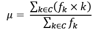
Here, k is the key from the Counter, C, and f_k is the frequency value for the given key from the Counter. The sum of all the frequencies is the total count of all the original samples.

The standard deviation, , depends on the mean, . The formula is this:

Here, k is the key from the Counter, C, and f_k is the frequency value for the given key from the Counter. The total number of items in the counter is .

How to do it...

1. Define the class with a descriptive name:

   class LazyCounterStatistics: 
   

2. Write the initialization method to include the object to which this object will be connected. We've defined a method function that takes a Counter object as an argument value. This counter object is saved as part of the Counter_Statistics instance:

       def __init__(self, raw_counter: Counter) -> None: 
           self.raw_counter = raw_counter 
   

3. Define some useful helper methods. Each of these is decorated with @property to make it behave like a simple attribute:

       @property
       def sum(self) -> float:
           return sum(
               f * v
               for v, f in self.raw_counter.items()
           )
       @property 
       def count(self) -> float: 
           return sum(
               f 
               for v, f in self.raw_counter.items()
           )
   

4. Define the required methods for the various values. Here's the calculation of the mean. This too is decorated with @property. The other methods can be referenced as if they are attributes, even though they are proper method functions:

       @property
       def mean(self) -> float:
           return self.sum / self.count
   

5. Here's how we can calculate the standard deviation. Note that we've been using math.sqrt(). Be sure to add the required import math statement in the Python module:

       @property
       def sum2(self) -> float:
           return sum(
               f * v ** 2 
               for v, f in self.raw_counter.items()
           )
       @property
       def variance(self) -> float:
           return (
               (self.sum2 - self.sum ** 2 / self.count) /
               (self.count - 1)
            )
       @property
       def stddev(self) -> float:
           return math.sqrt(self.variance)
   

To show how this works, we'll apply an instance of this class to the data created by the coupon collector function. The data from that function was organized as a Counter object that had the counts of visits required to get a full set of coupons. For each count of visits, the Counter instance kept the number of times it occurred. This provided a handy histogram showing a minimum and a maximum. The question we had was whether or not real data matched the statistical expectation.

Here's how we can create some sample data:

from Chapter_15.collector import * 
import collections
from typing import Counter, Callable, Iterator
ArrivalF = Callable[[int], Iterator[int]]
def raw_data(
    n: int = 8, 
    limit: int = 1000, 
    arrival_function: ArrivalF = arrival1
 -> Counter[int]:
    data = samples(limit, arrival_function(n))
    wait_times = collections.Counter(coupon_collector(n, data))
    return wait_times

We've imported functions such as expected(), arrival1(), and coupon_collector() from the Chapter_15.collector module. We've imported the standard library collections module. We've also imported the Counter type hint to provide a description the results of the raw_data() function.

We defined a function, raw_data(), that will generate a number of customer visits. The default for the resulting data will contain 1,000 visits. The domain will be eight different classes of customers; each class will have an equal number of members. We'll use the coupon_collector() function to step through the data, emitting the number of visits required to collect a full set of eight coupons.

This data is then used to assemble a Counter object. This will have the number of customers required to get a full set of coupons. Each number of customers will also have a frequency showing how often that number of visits occurred.

Here's how we can analyze the Counter object:

>>> import random
>>> random.seed(1)
>> data = raw_data(8)
>>> stats = LazyCounterStatistics(data)
>>> round(stats.mean, 2)
20.81
>>> round(stats.stddev, 2)
7.02

First, we imported the random module so that we could pick a known seed value. This makes it easier to test and demonstrate an application because the random numbers are consistent.

Setting the random number seed to a known value generates predictable, testable coupon collector test results. The results are randomized, but depend on the seed value. The raw_data() function will emit a Counter object, which we called data.

We'll use the Counter object to create an instance of the LazyCounterStatistics class. We'll assign this to the stats variable. When we print the value for the stats.mean property and the stats.stddev property, the methods are invoked to do the appropriate calculations of the various values.

For a set of eight coupons, the theoretical average is 21.7 visits to collect all coupons. It looks like the results from raw_data() show behavior that matches the expectation of random visits. This is sometimes called the null hypothesis—the data is random. Our customers are visiting us in nearly random orders, distributed fairly.

This might be a good thing because we've been trying to get a wider variety of customers to visit. It might be a bad thing because a promotional program has not moved the visits away from a random distribution. The subsequent decisions around this data depend on a great deal of context.

In this case, the generated data really was random. Using this is a way to validate the statistical testing approach. We can now use this software on real-world data with some confidence that it behaves correctly.

How it works...

The idea of lazy calculation works out well when the value is used rarely. In this example, the count is computed twice as part of computing the variance and standard deviation.

A naïve lazy design may not be optimal in some cases when values are recomputed frequently. This is an easy problem to fix, in general. We can always create additional local variables to cache intermediate results instead of recomputing them.

To make this class look like a class performing eager calculations, we used the @property decorator. This makes a method function appear to be an attribute. This can only work for method functions that have no argument values.

In all cases, an attribute that's computed eagerly can be replaced by a lazy property. The principle reason for creating eager attribute variables is to optimize computation costs. In the case where a value is used rarely, a lazy property can avoid an expensive calculation.

There's more...

There are some situations in which we can further optimize a property to limit the amount of additional computation that's done when a value changes. This requires a careful analysis of the use cases in order to understand the pattern of updates to the underlying data.

In the situation where a collection is loaded with data and an analysis is performed, we can cache results to save computing them a second time.

We might do something like this:

class CachingLazyCounterStatistics:
    def __init__(self, raw_counter: Counter) -> None:
        self.raw_counter = raw_counter
        self._sum: Optional[float] = None
        self._count: Optional[float] = None
    @property
    def sum(self) -> float:
        if self._sum is None:
            self._sum = sum(
                f * v
                for v, f in self.raw_counter.items()
            )
        return cast(float, self._sum)

This technique uses two attributes to save the results of the sum and count calculations, self._sum and self._count. This value can be computed once and returned as often as needed with no cost for recalculation.

The type hints show these attributes as being optional. Once the values for self._sum and self._count have been computed, the values are no longer optional, but will be present. We describe this to mypy with the cast() type hint. This hint tells mypy to consider self._sum as being a float object, not an Optional[float] object.

This caching optimization is only helpful if the state of the raw_counter object never changes. In an application that updates the underlying Counter, this cached value would become out of date. That kind of application would need to recreate the LazyCounterStatistics every time the Counter was updated.

See also...

• In the Designing classes with lots of processing recipe, we defined a class that eagerly computed a number of attributes. This represents a different strategy for managing the cost of the computation.

Creating contexts and context managers

A number of Python objects behave like context managers. Some of the most visible examples are file objects. We often use with path.open() as file: to process a file and guarantee the resources are released. In Chapter 2, Statements and Syntax, the recipe Context management and the "with" statement covers the basics of using a file-based context manager.

How can we create our own classes that act as context managers?

Getting ready

We'll look at a function from Chapter 3, Function Definitions, in the Picking an order for parameters based on partial functions recipe. This recipe introduced a function, haversine(), which has a context-like parameter used to adjust the answer from dimensionless radians to a useful unit of measure, such as kilometers, nautical miles, or US statute miles. In many ways, this distance factor is a kind of context, used to define the kinds of computations that are done.

What we want is to be able to use the with statement to describe an object that doesn't change very quickly; indeed the change acts as a kind of boundary, defining the scope of computations. We might want to use code like the following:

>>> with Distance(r=NM) as nm_dist:
...     print(f"{nm_dist(p1, p2)=:.2f}")
...     print(f"{nm_dist(p2, p3)=:.2f}")

The Distance(r=NM) constructor provides the definition of the context, providing a new object, nm_dist, that has been configured to perform the required calculation in nautical miles. This can be used only within the body of the with statement.

This Distance class definition can be seen as creating a partial function, nm_dist(). This function provides a fixed unit-of-measure parameter, r, for a number of following computations using the haversine() function.

There are a number of other ways to create partial functions, including a lambda object, the functools.partial() function, and callable objects. We looked at the partial function alternative in Chapter 3, Function Definitions, in the Picking an order for parameters based on partial functions recipe.

How to do it…

A context manager class has two special methods that we need to define:

1. Start with a meaningful class name:

   class Distance:
   

2. Define an initializer that creates any unique features of the context. In this case, we want to set the units of distance that are used:

       def __init__(self, r: float) -> None:
           self.r = r
   

3. Define the __enter__() method. This is called when the with statement block begins. The statement with Distance(r=NM) as nm_dist does two things. First it creates the instance of the Distance class, then it calls the __enter__() method of that object to start the context. The return value from __enter__() is what's assigned to a local variable via the as clause. This isn't always required. For simple cases, the context manager often returns itself. If this method needs to return an instance in the same class, the class hasn't been fully defined yet, and the class name has to be given as a string. For this recipe, we'll return a function, with the type hint based on Callable:

       def __enter__(self) -> Callable[[Point, Point], float]:
           return self.distance
   

4. Define the __exit__() method. When the context finishes, this method is invoked. This is where resources are released and cleanup can happen. In this example, nothing more needs to be done. The details of any exception are provided to this method; it can silence the exception or allow it to propagate. If the return value is True, the exception is silenced. False or None return values will allow the exception to be seen outside the with statement:

       def __exit__(
          self,
           exc_type: Optional[Type[Exception]],
           exc_val: Optional[Exception],
           exc_tb: Optional[TracebackType]
       ) -> Optional[bool]:
           return None
   

5. Create the class (or define the methods if an instance of this class is returned) that works within the context. In this case, we're using the haversine() function from Chapter 3, Function Definitions:

       def distance(self, p1: Point, p2: Point) -> float:
           return haversine(
               p1.lat, p1.lon, p2.lat, p2.lon, self.r
           )
   

This class requires a fairly large number of imports:

from types import TracebackType
from typing import Optional, Type, Callable, NamedTuple

This class has been defined to work with objects of the class Point. This can be a NamedTuple, dataclass, or some other class that provides the required two attributes. Here's the NamedTuple definition of Point:

class Point(NamedTuple):
    lat: float
    lon: float

Do remember, however, that this class works with any object of class Point.

How it works…

The context manager relies on the with statement doing a large number of things.

We'll put the following construct under a microscope:

>>> nm_distance = Distance(r=NM)
>>> with nm_distance as nm_calc:
...     print(f"{nm_calc(p1, p2)=:.2f}")

The first line creates an instance of the Distance class. This has a value for the r parameter equal to the constant NM, allowing us to do computations in nautical miles. The Distance instance is assigned to the nm_distance variable.

When the with statement starts execution, the context manager object is notified by having the __enter__() method executed. In this case, the value returned by the __enter__() method is a function, with the type Callable[[Point, Point], float]. The as clause assigns this object to the nm_calc variable.

The print() function does its work using the nm_calc object. This object is a function which will compute a distance from two Point instances.

When the with statement finishes, the __exit__() method will be executed. For more complex context managers, this may involve closing files or releasing network connections. There are a great many kinds of context cleanup that might be necessary. In this case, there's nothing that needs to be done to clean up the context.

This has the advantage of providing a fixed context boundary in which the partial function is being used. In some cases, the computation inside the context manager might involve a database or complex web services, leading to a more complex __exit__() method.

There's more…

The operation of the __exit__() method is central to making best use of a context manager. In the previous example, we use the following "do nothing" __exit__() method:

    def __exit__(
        self,
        exc_type: Optional[Type[Exception]],
        exc_val: Optional[Exception],
        exc_tb: Optional[TracebackType]
    ) -> Optional[bool]:
        # Cleanup goes here.
        return None

The point here is to allow any exception to propagate normally. We often see any cleanup processing replacing the # Cleanup goes here. comment. This is where buffers are flushed, files are closed, and error log messages are written. In more complex applications, the backup copy of a file may be restored.

Sometimes, we'll need to handle specific exception details. Consider the following snippet of an interactive session:

>>> p1 = Point(38.9784, -76.4922)
>>> p2 = Point(36.8443, -76.2922)
>>> with Distance(None) as nm_dist:
...     print(f"{nm_dist(p1, p2)=:.2f}")
Traceback (most recent call last):
    ...
TypeError: unsupported operand type(s) for *: 'NoneType' and 'int'

The Distance() class was initialized with the r argument value set to None. While this code will lead to warnings from mypy, it's syntactically valid. The type error traceback, however, doesn't point to the Distance class, but points to a line of code within the haversine() function.

We might want to report a ValueError instead of this TypeError. Here's a variation on the Distance class, called Distance_2. This class conceals the TypeError, replacing it with a ValueError:

class Distance_2:
    def __init__(self, r: float) -> None:
        self.r = r
    def __enter__(self) -> Callable[[Point, Point], float]:
        return self.distance
    def __exit__(
        self,
        exc_type: Optional[Type[Exception]],
        exc_val: Optional[Exception],
        exc_tb: Optional[TracebackType]
    ) -> Optional[bool]:
        if exc_type is TypeError:
            raise ValueError(f"Invalid r={self.r}")
        return None
    def distance(self, p1: Point, p2: Point) -> float:
        return haversine(p1.lat, p1.lon, p2.lat, p2.lon, self.r)

This shows how we can examine the details of the exception in the __exit__() method. The information provided parallels the sys.exc_info() function, and includes the exception's type, the exception object, and a traceback object with the types.TracebackType type.

See also

• In the Context management and the "with" statement recipe in Chapter 2, Statements and Syntax, we cover the basics of using a file-based context manager.

Managing multiple contexts with multiple resources

We often use context managers with open files. Because the context manager can guarantee the OS resources are released, doing so prevents resource leaks and files that are damaged from being closed without having all of the bytes properly written to persistent storage.

When multiple resources are being processed, it often means multiple context managers will be needed. If we have two or three open files, does this mean we have deeply nested with statements? How can we optimize or simplify multiple with statements?

Getting ready

We'll look at creating a plan for a journey with multiple legs. Our starting data collection is a list of points that define our route. For example, traveling through Chesapeake Bay may involve starting in Annapolis, Maryland, sailing to Solomon's Island, Deltaville, Virginia, and then Norfolk, Virginia. For planning purposes, we'd like to think of this as three legs, instead of four points. A leg has a distance and takes time to traverse: the time and distance are the essence of the planning problem.

We'll start with some foundational definitions before we run the recipe. First is the definition of a single point, with attributes of latitude and longitude:

@dataclass(frozen=True)
class Point:
    lat: float
    lon: float

A point can be built with a statement like this: p = Point(38.9784, -76.4922). This lets us refer to p.lat and p.lon in subsequent computations. The use of attribute names makes the code much easier to read.

A leg is a pair of points. We can define it as follows:

@dataclass
lass Leg:
    start: Point
    end: Point
    distance: float = field(init=False)

We've created this as a mutable object. The distance attribute has an initial value defined by the dataclasses.field() function. The use of init=False means the attribute is not provided when the object is initialized; it must be supplied after initialization.

Here's a context manager to create Leg objects from Point instances. This is similar to the context managers shown in the Using contexts and context managers recipe. There is a tiny but important difference here. The __init__() saves a value for self.r to set the distance unit context. The default value is nautical miles:

class LegMaker:
    def __init__(self, r: float=NM) -> None:
        self.last_point: Optional[Point] = None
        self.last_leg: Optional[Leg] = None
        self.r = r
    def __enter__(self) -> 'LegMaker':
        return self
    def __exit__(
        self,
        exc_type: Optional[Type[Exception]],
        exc_val: Optional[Exception],
        exc_tb: Optional[TracebackType]
    ) -> Optional[bool]:
        return None

The important method, waypoint(), accepts a waypoint and creates a Leg object. The very first waypoint, the starting point for the voyage, will return None. All subsequent points will return a Leg object:

def waypoint(self, next_point: Point) -> Optional[Leg]:
    leg: Optional[Leg]
    if self.last_point is None:
        # Special case for the first leg
        leg = None
    else:
        leg = Leg(self.last_point, next_point)
        d = haversine(
            leg.start.lat, leg.start.lon, 
            leg.end.lat, leg.end.lon, self.r
        )
        leg.distance = round(d)
    self.last_point = next_point
    return leg

This method uses a cached point, self.last_point, and the next point, next_point, to create a Leg instance.

If we want to create an output file in CSV format, we'll need to use two context managers: one to create Leg objects, and another to manage the open file. We'll put this complex multi-context processing into a single function.

How to do it…

1. Define the headers to be used for the CSV output:

   HEADERS = ["start_lat", "start_lon", "end_lat", "end_lon", "distance"]
   

2. Define a function to transform complex objects into a dictionary suitable for writing each individual row. The input is a Leg object; the output is a dictionary with keys that match the HEADERS list of column names:

   def flat_dict(leg: Leg) -> Dict[str, float]:
       struct = asdict(leg)
       return dict(
           start_lat=struct["start"]["lat"],
           start_lon=struct["start"]["lon"],
           end_lat=struct["end"]["lat"],
           end_lon=struct["end"]["lon"],
           distance=struct["distance"],
       )
   

3. Define the function with a meaningful name. We'll provide two parameters: a list of Point objects and a Path object showing where the CSV file should be created. We've used Iterable[Point] as a type hint so this function can accept any iterable collection of Point instances:

   def make_route_file(
       points: Iterable[Point], target: Path
   ) -> None:
   

4. Start the two contexts with a single with statement. This will invoke both __enter__() methods to prepare both contexts for work. This line can get long, and parentheses can't easily be used to extend it, so a is often used for complex with statements:

       with LegMaker(r=NM) as legger, 
           target.open('w', newline='') as csv_file:
   

5. Once the contexts are ready for work, we can create a CSV writer and begin writing rows:

       writer = csv.DictWriter(csv_file, HEADERS)
       writer.writeheader()
       for point in points:
           leg = legger.waypoint(point)
           if leg is not None:
               writer.writerow(flat_dict(leg))
   

6. At the end of the context, do any final summary processing. This is not indented within the with statement's body; it is at the same indentation level as the with keyword itself:

   print(f"Finished creating {target}")
   

How it works…

The compound with statement created a number of context managers for us. All of the managers will have their __enter__() methods used to both start processing and, optionally, return an object usable within the context. The LegMaker class defined an __enter__() method that returned the LegMaker instance. The Path.open() method returns a TextIO object; these are also context managers.

When the context exits at the end of the with statement, all of the context manager __exit__() methods are called. This allows each context manager to do any finalization. In the case of TextIO objects, this closes the external files, releasing any of the OS resources being used. In the cast of the LegMaker object, there is no finalization processing on context exit.

There's more…

A context manager's job is to isolate details of resource management. The most common examples are files and network connections. We've shown using a context manager around an algorithm to help manage a cache with a single Point object.

In this example, we specifically strove to avoid accumulating a large number of Leg instances. For some kinds of data science applications, the entire dataset doesn't fit in memory, and it's challenging to work with all the data in a single list or pandas DataFrame.

When working with very large datasets, it's often helpful to use compression. This can create a different kind of context around the processing. The built-in open() method is generally assigned to the io.open() function in the io module. This means we can often replace io.open() with a function such as bz2.open() to work with compressed files.

We can replace the context manager with something like this:

def make_route_bz2(
    points: Iterable[Point], target: Path
) -> None:
    with LegMaker(r=NM) as legger, 
            bz2.open(target, "wt") as archive:
        writer = csv.DictWriter(archive, HEADERS)
        writer.writeheader()
        for point in points:
            leg = legger.waypoint(point)
            if leg is not None:
                writer.writerow(flat_dict(leg))
    print(f"Finished creating {target}")

We've replaced the original path.open() method with bz2.open(path). The rest of the context processing remains identical. This flexibility allows us to work with text files initially and convert to compressed files when the volume of data grows or when we move away from testing and experimenting into full-sized production use of the software.

See also

• In the Context management and the "with" statement recipe in Chapter 2, Statements and Syntax, we cover the basics of using a file-based context manager.
• The Creating contexts and context managers recipe covers the core of creating a class that is a context manager.