12. Spreadsheets with Numbers

With Numbers, you can create data spreadsheets, perform calculations, and create forms and charts.
![]() Calculating Totals and Averages
Calculating Totals and Averages
Numbers is a versatile program that enables you to create the most boring table of numbers ever (feel free to try for the world record on that one) or an elegant chart that illustrates a point like no paragraph of text ever could.
Creating a New Spreadsheet
The way you manage documents in Numbers is exactly the same as you do in Pages, so if you need a refresher, refer to Chapter 11, “Writing with Pages.” Let’s jump right in to creating a simple spreadsheet.
1. Tap the Numbers icon on your Home screen to start.
2. Tap + and then Create Spreadsheet to see all the template choices.
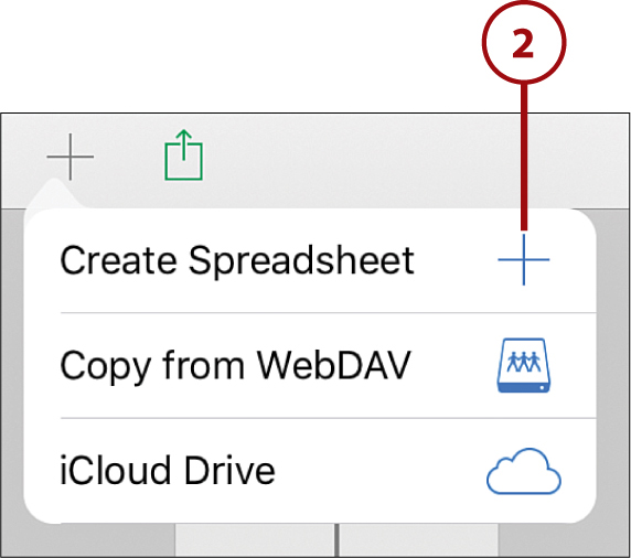
3. Tap Blank to choose the most basic template.

Numbers Terminology
A grid of numbers is called a table. A page of tables, often just a single table taking up the whole page, is a sheet. You can have multiple sheets in a document, all represented by tabs. The first tab in this case represents “Sheet 1.” Tap the + to add a new sheet.
4. Tap in one of the cells to select the sheet. An outline appears around the cell.

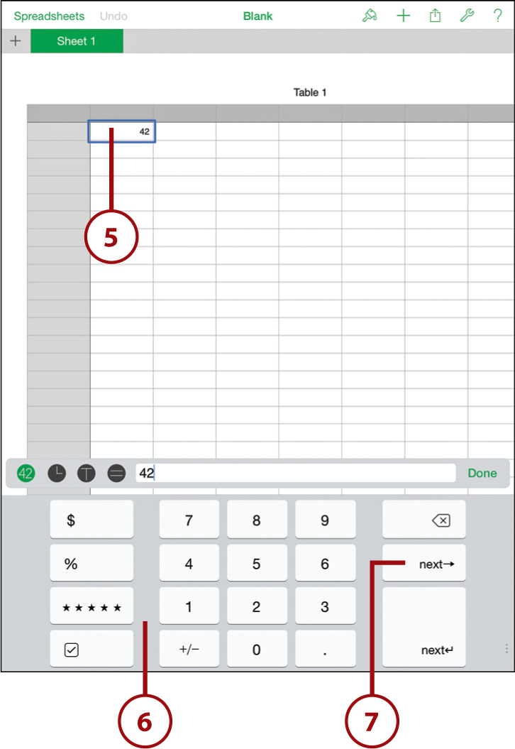
5. Double-tap the cell this time. An on-screen keypad appears.
6. Use the keypad to type a number. The number appears in both the cell and a text field above the keypad. Use this text field to edit the text, tapping inside it to reposition the cursor if necessary.
7. Tap the upper Next button, the one with the arrow pointing right.
Switching Keyboard Options
The four buttons just above and to the left of the keypad represent number, time, text, and formula formats for cells. If you select the number, you get a keypad to enter a number. If you select the clock, you get a special keypad to enter dates and times. If you select the T, you get a regular keyboard. Finally, if you select the equal sign (=), you get a keypad and special buttons to enter formulas.
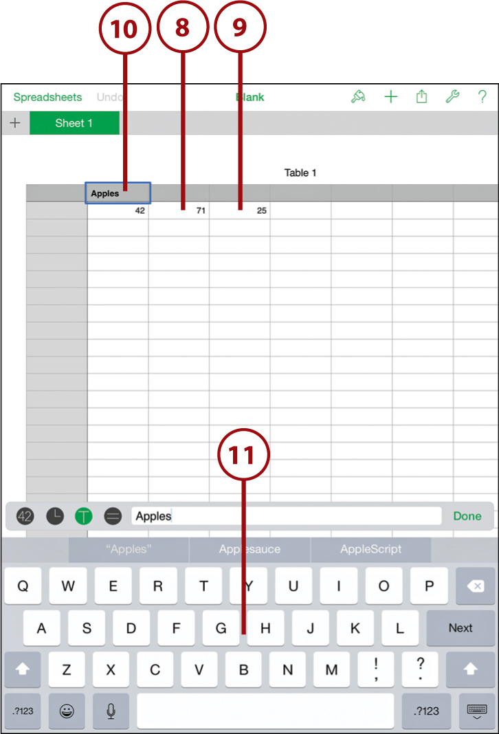
8. The cursor moves to the column in the next cell. Type a number here, too.
9. Tap the Next button again and enter a third number.
10. Tap the space just above the first number you entered. The keypad changes to a standard keyboard to type text instead of numbers.
11. Type a label for this first column.
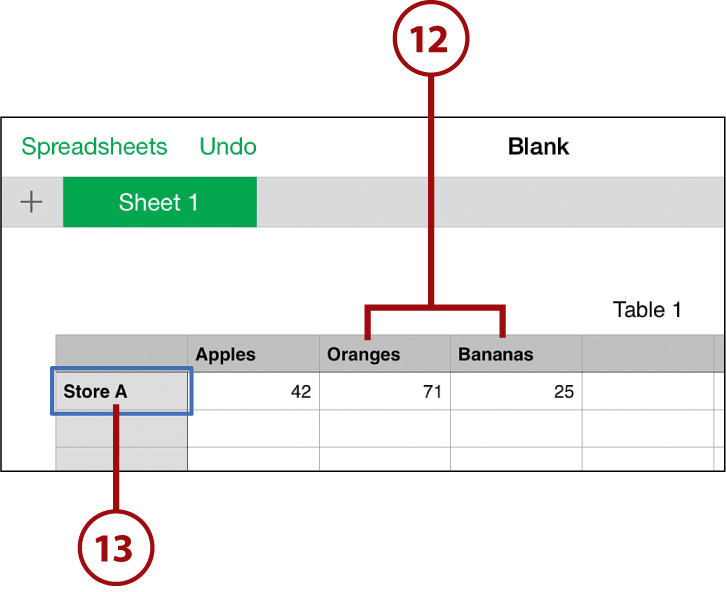
12. Tap in each of the other two column heads to enter titles for them as well.
13. Tap to the left of the first number you entered. Type a row title.
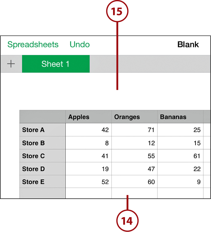
14. Now enter a few more rows of data.
15. Tap the Done button or tap outside of the table to dismiss the keyboard.
16. Tap any cell in the table to select the table.
17. Tap and drag the circle with two lines in it to the right of the bar above the table. Drag it to the left to remove the unneeded columns. To do this, you might need to drag the whole screen to bring the right side of the table into view.
18. Tap and drag the same circle at the bottom of the vertical bar to the left of the table. Drag it up to remove most of the extra rows, leaving two at the bottom for future use.

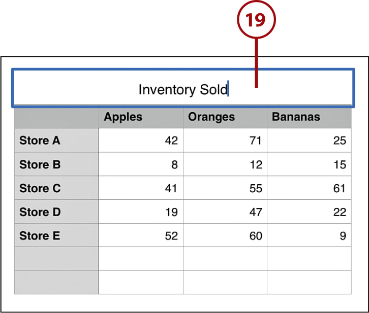
19. Double-tap the title of the table and give it a name.
Calculating Totals and Averages
One of the most basic formula types is a sum. In the previous example, for instance, you might want to total each column. You might also want to find the average of the numbers in the columns.
With tables, you typically put these kinds of calculations in footer rows. So, your table has header rows with the title of each column and footer rows with things like sums and averages.
1. Start with the result of the previous example. Select any cell in the table. Then tap the paintbrush to bring up the controls.
2. Tap the Headers tools.
3. Increase the number of Footer Rows to 2. This turns the last two rows in the table to footer rows.

You can put a formula to perform calculations in any cell of a table. So why bother with footer rows? They give you two nice features. First, you can now ask for the sum or average of an entire column, and Numbers knows to not include values in header and footer rows. Second, if you are entering values in the last cell of the last row above a footer row, and you tap the New key on the keyboard, Numbers inserts a new row and automatically moves the footer rows down.
4. Double-tap in the cell just below the bottom number in the first column.
5. Tap the = button to switch to the formula keypad.

6. Tap the SUM button on the keypad.
7. The formula for the cell appears in the text field. Because you are using a footer row, Numbers automatically assumes you want the sum of this column, so it puts the name of the column into the formula. Otherwise, you would have to tap the column letter at the top of the column, manually enter “B,” or select a range of cells such as “B2:B6” for the formula.
8. The result of the formula instantly appears in the spreadsheet.
9. Tap the green check mark button to dismiss the keyboard.

10. Repeat steps 2 through 4 for the other columns in the table.

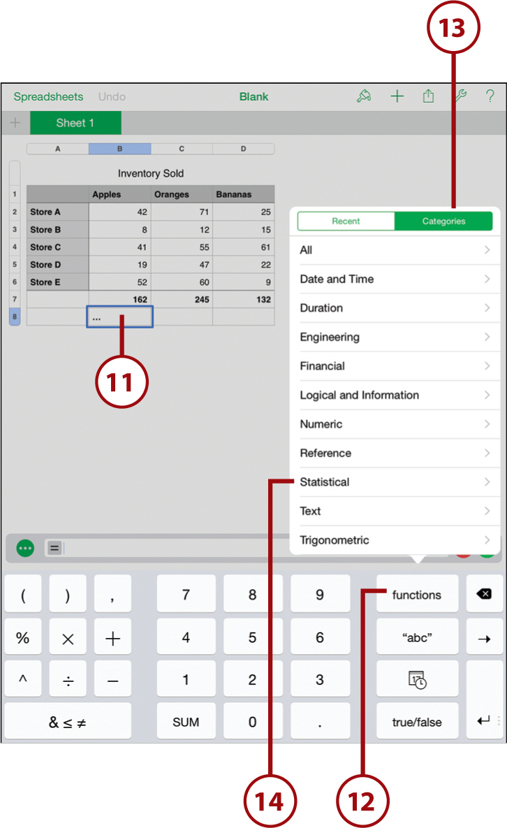
11. Double-tap the last cell in the first column.
12. Tap the = button like you did in step 5, but this time tap the Functions button instead of SUM. This brings up the Functions menu.
13. Tap Categories at the top of the Functions menu.
14. Tap Statistical to dig down into those functions, and then tap AVERAGE in the list that appears.
15. This time we need to give the AVERAGE function a range to work with, as it doesn’t do it automatically like SUM did. Tap the B at the top of the column. This should fill in the function with “Apples,” as that is the name of column B.
16. Tap the check mark to dismiss the keyboard and complete the formula.

17. Do the same for the next two columns. Or, you can select the first cell, copy it, then paste it into the second and third. When you do, select Paste Formula so the formula, and not the value, is pasted. The references to the columns shift automatically so each averages the appropriate column.
18. You can also enter labels for these two footer rows.

Automatic Updates
If you are not familiar with spreadsheets, the best thing about them is that formulas like this automatically update. So if you change the number of Apples in Store C in the table, the sum in the last row automatically changes to show the new total.
Styling Tables and Cells
When working with tables, you can assign many different style options. It is easy to set the style for an entire table, but you can also make design choices for a single cell or group of cells.
1. Start with a table like the one we have been working with in the previous tasks. Select any cell in it.
2. Tap the paintbrush button.
3. Select Table.
4. Select a style. You see it reflected in the table immediately.
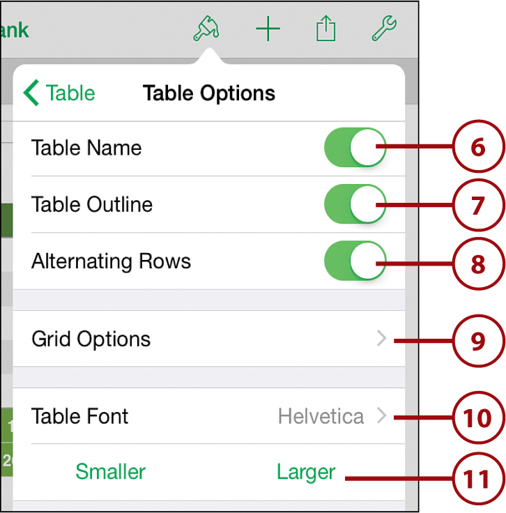
5. Tap Table Options to customize the table design.

6. You can switch off the table name so it is no longer visible.
7. You can switch off the thin outline that surrounds the entire table.
8. Rows in the table normally alternate between light and dark background shades to make it easier to read. You can turn this off as well.
9. Grid Options lets you decide where lines appear between cells.
10. You can change the font used by the table.
11. You can easily make the text larger or smaller.
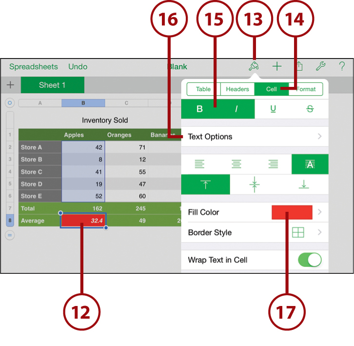
12. Select a single cell or group of cells. In this case, select a cell to highlight to point out something in the table.
13. Tap the paintbrush button.
14. Tap Cell.
15. Tap any of the style buttons at the top to apply a style, such as italic.
16. Tap Text Options to change the size, color, and font.
17. Tap the Fill Color to change the background color of the cell.
18. Tap Format.
19. This menu allows you to set a format for the cell. For instance, you could choose Currency, and a currency symbol, such as $, would be placed before the number. There are a wide variety of different formats to choose from.

Creating Forms
Forms are an alternative way to enter data in a spreadsheet. A form contains many pages, each page representing a row in a table. Continue with the previous example and use it to make a form.
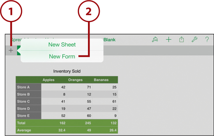
1. Tap the + button in the upper-left corner.
2. Tap New Form. Note that in order to get the option to make a form, you need to have at least one column with a value in its header row.
3. Choose a table. We have only one, so the choice is simple. Tap Table 1 to see the first page in the form, which represents the first row of data from our table.

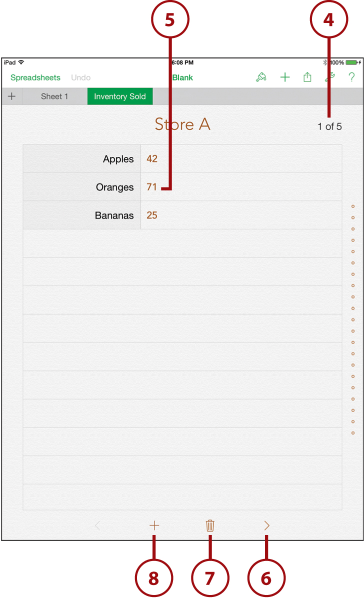
4. The form appears. It shows one record, or row of the table, at a time. You can see which row it is showing and the total number of rows. Note that header and footer rows are not included—only the rows in the main body of the table.
5. You can tap any value and change it.
6. Tap the right arrow at the bottom of the screen to move through the five existing rows (pages) of data.
7. If you want to delete any row, tap the trash can button.
8. Tap the + button at the bottom of the screen to enter a new row of data after the one you are currently viewing. So if you want to add to the bottom of the table, go to the last page of the form first.
9. Tap at the top of the screen to enter a row heading.
10. Tap in each of the three fields to enter data.

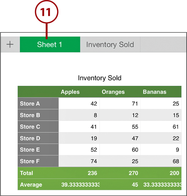
11. When you finish, tap the first tab, Sheet 1, to return to the original spreadsheet. You should see the new data in a new row. The totals and averages have updated as well.
Using Multiple Tables
The primary way Numbers differs from spreadsheet programs such as Excel is that Numbers emphasizes page design. A Numbers sheet is not meant to contain just one grid of numbers. In Numbers, you can use multiple tables. By using multiple tables, you can track data more efficiently. Let’s look at an example.
1. Continuing with the example you have been building, keep the current table and move it down to make space for another. Tap the + button to add a second table.
Selecting a Table
It can be difficult to select an entire table without selecting a cell. Tap in a cell to select it. Then tap the circle that appears in the upper-left corner of the table to change your selection to the entire table.
2. Using what you have learned in this chapter so far, create a small second table with prices as shown.
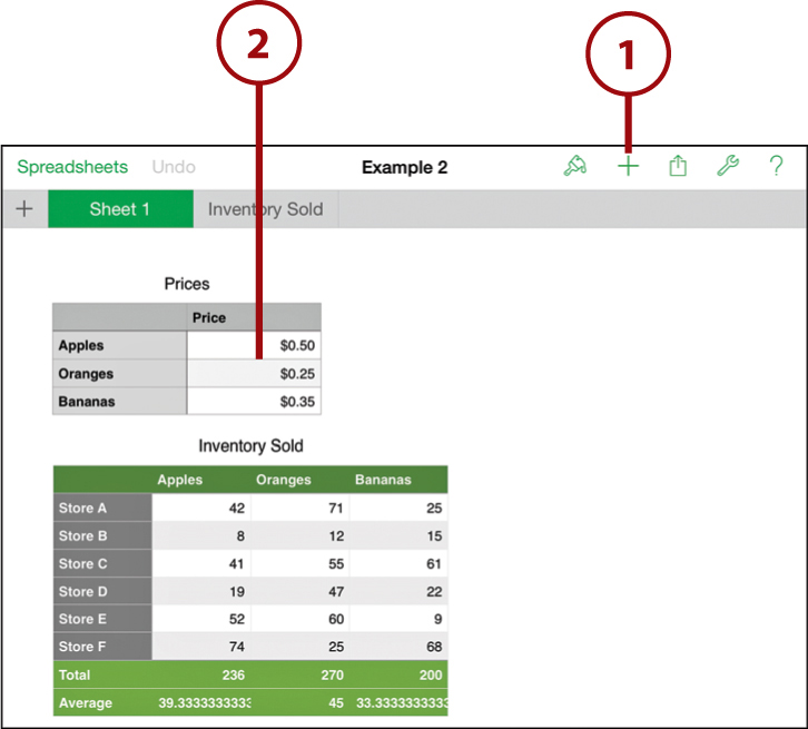
3. Expand the original table by adding one more column.
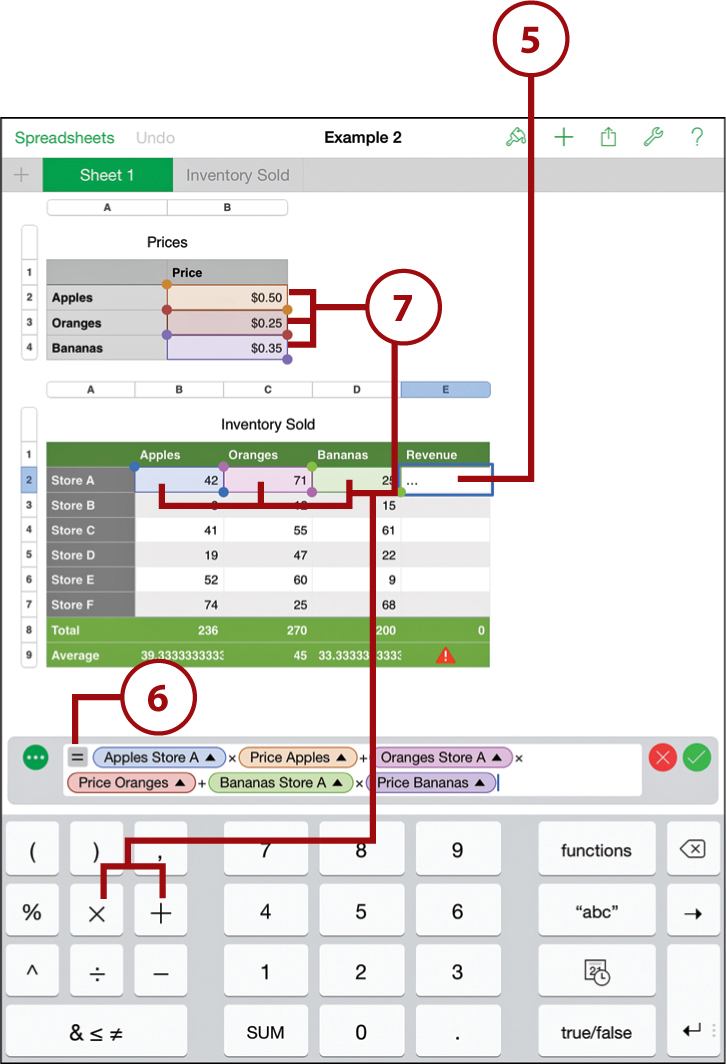
4. Name this column Revenue. Notice that when you expand the table, the total and average formulas in the footer columns are automatically added. The average now gives an error because it is attempting to find the average of an empty column.

5. Double-tap the first empty cell in the new column to bring up the keyboard.
6. Tap the = button to start entering a formula.
7. You want to multiply the number of items in each cell by the price that matches it. Tap the cell that represents Apples from Store A, tap the X symbol on the keyboard, and then tap the cell that represents the price of Apples in the upper table. Tap + in the keyboard and do the same for Oranges and Bananas.
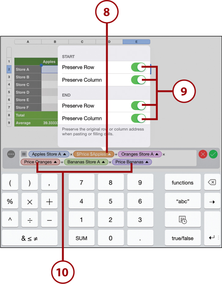
8. The plan is to copy and paste this formula into all rows. When you do that, the references in the formula change to match the relative position of the cell it is being pasted into. You want that for the Inventory numbers, but you don’t want that for the prices. You want those to stay fixed. So tap the Price Apples item in the formula to bring up a menu.
9. Switch on all Preserve options for this item. This ensures that as you paste the formula elsewhere, it always points to the price of apples in the upper table.
10. Do the same for Price Oranges and Price Bananas.
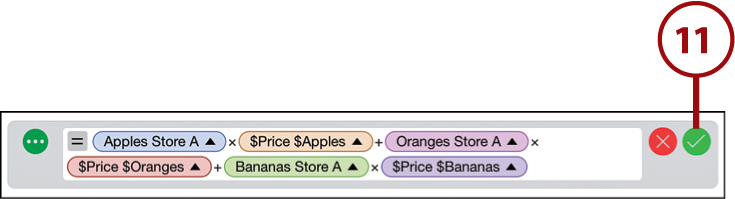
11. The formula should now look like this. Notice the $ symbol is used to indicate that a reference is absolute and not relative to the position of the formula. Tap the green check mark to finish the formula.
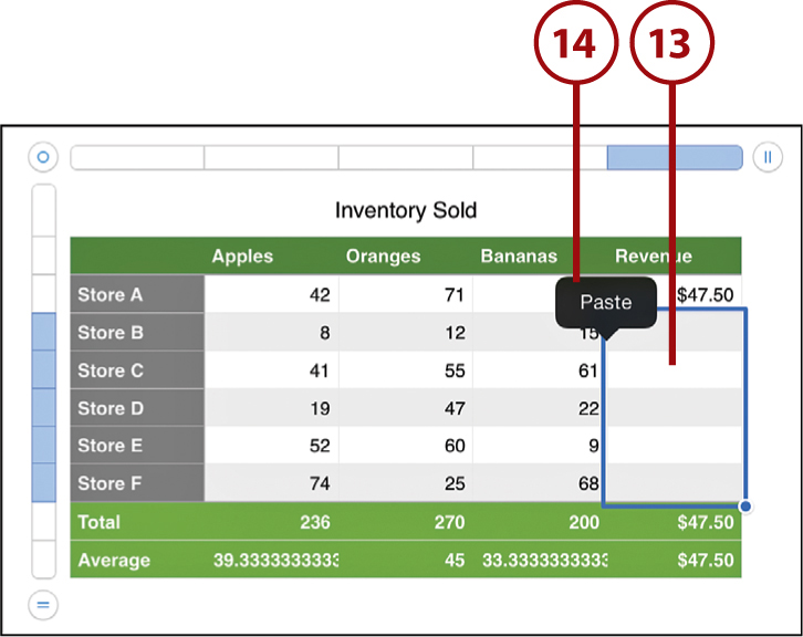
12. Tap to select this cell and then tap Copy from the context menu.

13. Tap the next cell, and then expand the selection to include all the empty cells in that column.
14. Tap Paste in the context menu that should appear.
15. Tap Paste Formulas.
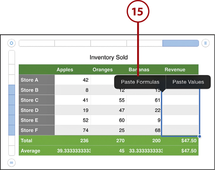
16. The values for all the rows are calculated.
17. Note that the total and averages are calculated as well.
18. If you change one of the prices in the upper table, all the values for revenue change instantly to reflect it.

Enhance the Sheet
Another thing you can do is add more titles, text, and images to the sheet—even shapes and arrows. These not only make the sheet look nice, but can also act as documentation as a reminder of what you need to do each month—or instruct someone else what to do to update the sheet.
Creating Charts
Representing numbers visually is one of the primary functions of a modern spreadsheet program. With Numbers, you can create bar, line, and pie charts and many variations of each.
1. Start with a table similar to the one you have been working with in this chapter. Select the whole table. Numbers uses the header column and header row, along with the numbers in the body of the table, to build the chart.
2. Tap the + button.
3. Select charts.
4. You can select 2D, 3D, or Interactive charts. For this example, stick with a simple 2D chart. But take the time to explore the others as well.
5. You can swipe horizontally to see different chart styles. There are several pages of them.
6. Tap a chart to insert it into your sheet.
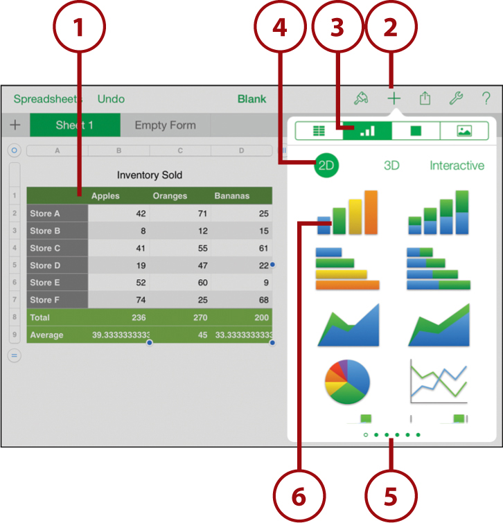
7. A chart is created using the data from your table. In this case, each store is represented along the horizontal axis, with a bar for each product. The vertical axis shows you the number sold.

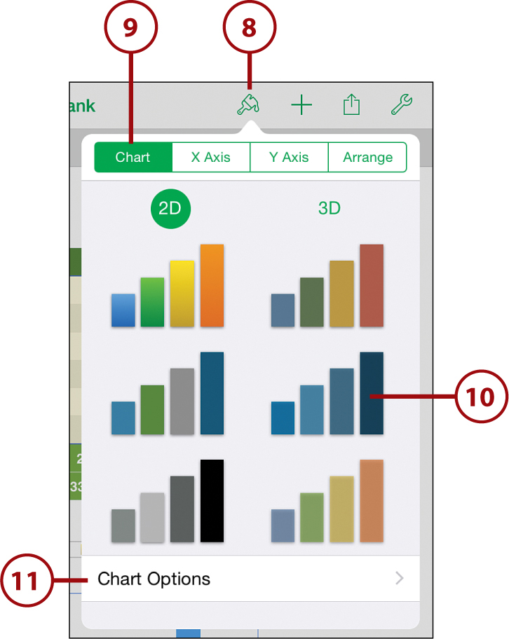
8. With the chart selected, tap the paintbrush button.
9. Tap Chart.
10. You can select a different style for the chart.
11. Tap Chart Options.
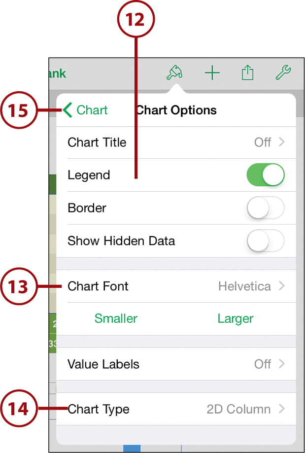
12. In the Chart Options controls, you can turn various elements on or off.
13. You can also customize the text in the chart.
14. You can even switch chart types.
15. Tap Chart to return to the previous set of controls.
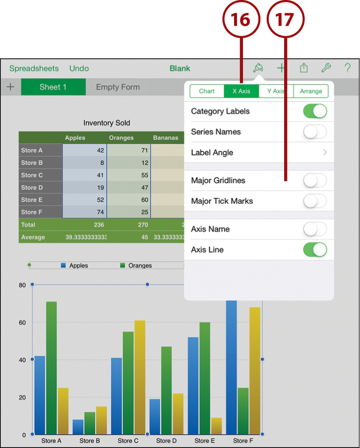
17. You can turn off various portions of the chart related to the selected axis.
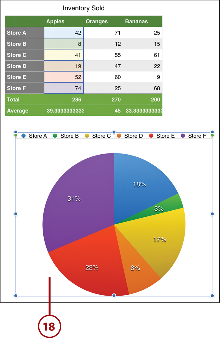
18. So what happens if you choose a different type of chart? Numbers tries its best to match the data to the chart. If you choose a pie chart, only one column of data is used. You can see when the chart is selected that the table above it uses colors to show which cell matches which slice of the pie.