
2
Morphological Characterization Techniques for Nano-Reinforced Polymers
Adoté Sitou BLIVI1, Benhui FAN2, Djimédo KONDO3 and Fahmi BEDOUI1
1 Université de technologie de Compiègne, Sorbonne University, France
2 CentraleSupélec, Paris-Saclay University, Gif-sur-Yvette, France
3 Institut Jean Le Rond d’Alembert, Sorbonne University, Paris, France
Nano-reinforced polymers are considered to be heterogeneous materials for which the heterogeneity is of nanometric size. In this case, their morphological characterization requires the use of experimental tools that are capable of investigating these scales. The microstructure characterization techniques that can meet this requirement are transmission electron microscopy (TEM) and X-ray diffraction (XRD) at small and wide angles. These two observation techniques are complementary. Indeed, TEM ensures a global and direct observation of the microstructure while XRD allows a so-called indirect observation, at smaller scales than TEM. XRD makes it possible to determine characteristic parameters which can be inaccessible to the TEM, such as intermolecular and intramolecular distances.
2.1. Transmission electron microscopy
Among the 2D observation techniques of the microstructure of polymer matrix nanocomposites, TEM seems to be the most suitable. It enables a direct observation of the microstructure with a sufficiently accurate resolution to determine the size of nanoparticles and aggregates. TEM observations require the preparation of samples that are adapted to nano-reinforced polymers. After observation, image processing is necessary to determine the microstructure parameters.
2.1.1. Sample preparation and acquisition of the TEM images
Before any manipulation, the samples used for the TEM observations are taken from the core of the material (the useful part of the specimen). For the observations, the samples are cut into very thin slices with a thickness between 70 and 100 nm in water using a Leica EM UC7 ultramicrotome with a Diatome ultra 45° diamond. The slices are then placed on 300-mesh copper grids and baked at 40°C for 5 min to remove any trace of moisture. The grids are then placed in the microscope for observation. The microscope used is a JEOL-JSM-2100F with an acceleration voltage of 200 kV. During the observation, the slice of material is bombarded by an electron beam that loses energy depending on the density of the area traversed, resulting in a density-dependent gray-scale image on output. The silica nanoparticles have a higher density than the poly(methyl methacrylate) (PMMA); we therefore obtain an image in which the nanoparticles are represented by dark areas (Figures 2.1 and 2.2). Being exposed to the beam can cause the slice to heat, and therefore it is cooled with liquid nitrogen during observation.
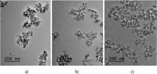
Figure 2.1. Snapshots of nanocomposites with 25 nm nanoparticles for volume fractions of a) 2%, b) 4% and c) 6%
Figures 2.1 and 2.2 represent, respectively, the images of nanocomposites with 25 nm and 150 nm nanoparticles for volume fractions of 2%, 4% and 6%. In these figures, it can be noticed that, for the same scale of observation and the same particle size, the particle density increases with the volume fraction. We can also notice that the dispersion state decreases with the decrease in the nanoparticle size. At a fixed nanoparticle size, the number of nanoparticles increases with increasing volume fraction. By comparing the images in Figure 2.1 with those in Figure 2.2, we can already notice that the dispersion in the case of large particles is better than that of small particles.

Figure 2.2. Snapshots of nanocomposites with 150 nm nanoparticles for volume fractions of a) 2%, b) 4% and c) 6%
2.1.2. Size, dispersion and interparticle distance
The collection of information (nanoparticle and aggregate size, dispersion rate and interparticle distance) on the microstructure of the nanocomposites was done by image processing, using the free software ImageJ (Rasband 2012), of the pictures obtained by TEM. It consists of the removal of the shadow areas by means of uniform illumination of the images, followed by a binarization and an analysis of the particles. This process is achieved in several steps. The goal of the processing is to eliminate the contribution of the matrix and to recover the contribution of the nanoparticles without degrading the contours. In Figure 2.3(a), which corresponds to the original image, one can note that the upper left corner is less illuminated than the lower right corner. The first step of the process consists of removing the shadows and illuminating the image in a uniform way to separate the contrast of the nanoparticles from that of the matrix based on the gray levels (Figure 2.3(b)). This contrast separation is done using the bandpass filter implemented in the ImageJ software. The image is then binarized and the residuals of the matrix are removed by the noise tool (Figure 2.3(c)). At this stage, only the contribution of the nanoparticles remains on the image. The final image (Figure 2.3(d)) is then analyzed for nanoparticle detection. Using the nanoparticle analysis tool available in ImageJ, the surfaces of the detected nanoparticles were recorded, as was the position of their center of mass (coordinates of the center of gravity of the nanoparticle). The detection of the coordinates is done by scanning the image along the x and y axes. On each axis, the scan is done pixelwise. Due to the binarization, all that remains in the image are gray levels that are close to white (255) and those that are close to black (0 nanoparticles). As a result, the contours and surfaces of nanoparticles and aggregates were determined.
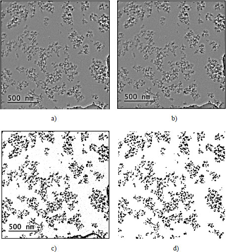
Figure 2.3. Image analysis with Image J: a) raw image, b) removal of shadow areas and uniform illumination, c) matrix removal and d) removal of the matrix residues
The surfaces of the nanoparticles were used to calculate their gyration diameter, which we assimilated to the diameter and dispersion rate within the matrix. We wrote a routine in Matlab® to calculate the distance between a nanoparticle and its nearest neighbor by the principle presented in Figure 2.4. The input data of the routine are the positions (coordinates) obtained by the analysis of the particles with the ImageJ software. The principle of the routine consists of calculating the distance between each pair of nanoparticles formed by a nanoparticle of fixed position and another one that can be seen in the picture. It then calculates the difference between the distance of each pair of nanoparticles and the sum of their radii. The interparticle distance is the minimum of these differences. These calculations are repeated for all the nanoparticles present on the plate and for each type of nanocomposite, and the number of plates processed per size is between 6 and 12. For large particles that are well dispersed, six TEM images were sufficient, because they have fairly close dispersion rates. On the other hand, for small particles, up to 12 images were sometimes processed. Increasing the number of images makes it possible to increase the population size and reduce variations from the mean.
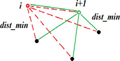
Figure 2.4. Diagram of the determination of the nearest neighbor distance using the Matlab® code. For a color version of this figure, see www.iste.co.uk/bai/nanocomposites.zip
The frequencies of nanoparticle size occurrence and interparticle distances are then approximated with a log-normal function. We consider the mean of the log-normal function as the mean of the treated population. The nanoparticle dispersion rate is the percentage corresponding to the mean of the nanoparticle sizes. The size distribution in log-normal function will be used in Chapter 4 for estimating the properties with the micromechanical model.
Figure 2.5 plots the frequency of occurrence (left axis) and the cumulative dispersion rate (right axis) of the 25 nm and 150 nm nanoparticle size for the 2%, 4% and 6% volume fractions. The average nanoparticle size is the center of the log-normal curve (red curve) and the average dispersion rate is the percentage dispersion corresponding to the average. As an example, for the 2%/25 nm nanocomposites, the average size is 26 nm and the corresponding dispersion rate is 67%. “n” is the number of nanoparticles or aggregates used to draw the curve. The analysis of these curves allowed the sizes of the nanoparticles and aggregates to be determined. Therefore, for nanoparticles with theoretical diameters of 25 nm and 150 nm, diameters of 26 nm and 170 nm were measured on average, respectively (Table 2.1). The analysis also helped to determine the size of the aggregates that are particularly present in the case of small nanoparticles. Figure 2.5 also shows the average dispersion rate corresponding to the average size of the nanoparticles. A decrease in the dispersion rate can be observed with the decrease in the size of the nanoparticles. Indeed, for a volume fraction of 2%, the dispersion rate is 67% and 74%, respectively, for 25 nm and 150 nm nanoparticles. This rate is 35% for 15 nm nanoparticles at 2% (see Table 2.1), where aggregates are particularly prevalent. The same observation is made for the other volume fractions. Nanoparticles tend to agglomerate as their size decreases, which reduces the dispersion rate. The agglomeration of small-sized nanoparticles is due to surface tension and their ability to attract each other, which increases as their size decreases (Cheng et al. 1993; Banfield and Zhang 2001). The smaller the size of the nanoparticles, the greater the attraction field surrounding them. The choice of combining solution and melt-mixing techniques seems to pay off rather well for dispersing nanoparticles, except for 15 nm nanoparticles. For the other sizes, we obtained more than 60% good dispersion, which is encouraging considering the gap between the nanoparticle scale and the scale at which we work.
By processing the images, it was also possible to determine the interparticle distance, which is the average of the distances between a nanoparticle and its closest neighbor. At constant volume fraction, these distances are a function of the particle sizes. Figure 2.6 shows the distribution of the interparticle distance in nanocomposites with 25 nm and 150 nm diameter nanoparticles for volume fractions of 2%, 4% and 6%. The average interparticle distance is the center of the log-normal curve. The values of the interparticle distances are recorded in Table 2.1. In general, a decrease in interparticle distance is observed with the decreasing size of nanoparticles with fixed volume fraction. A decrease in this distance is also observed when the volume fraction is increased at fixed nanoparticle size. As a matter of fact, at constant volume fraction the number of nanoparticles increases when the size of the nanoparticles decreases. This results in decreasing distances. This decrease in the interparticle distance will reduce the matrix chain mobility and thus lead to a limitation. The limitation will result in changes in the properties of the matrix, which will be discussed in Chapter 3 (Shin et al. 2015; Tessema et al. 2017).
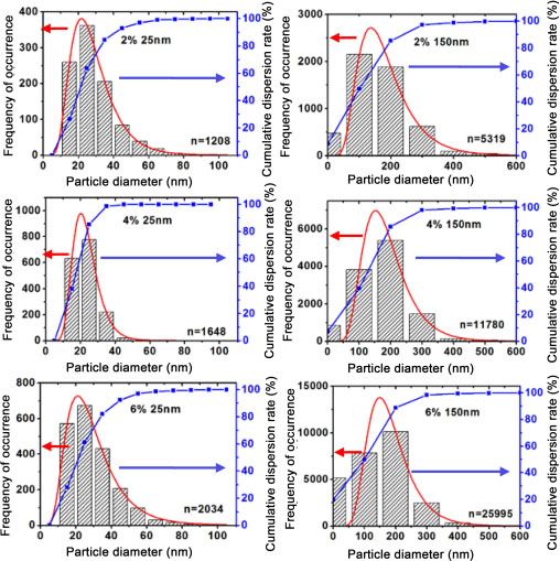
Figure 2.5. Size distribution and dispersion of 25 nm and 150 nm nanoparticles within the matrix for the volume fractions of 2%, 4% and 6%. For a color version of this figure, see www.iste.co.uk/bai/nanocomposites.zip
TEM observations have enabled an observation of the microstructure. They first made it possible to verify the spherical size of the fillers and their dimensions. The rate of aggregates present in the microstructure is significant in the case of small size nanoparticles despite the efforts made to disperse them well. The derived information could be used as input in a modeling approach. These observations can also then help to quantify the size effects on the microstructure.
The size effect not only concerns the size of the nanoparticles and aggregates, their dispersion and interparticle distances but also the behavior of the matrix with respect to the size of the nanoparticles. Microstructure parameters related to the nanoparticles were determined through the TEM analyses.
However, the microstructural parameters of the matrix cannot be determined by TEM observations. In order to access them, we will use the experimental technique adapted to the matrix, which is X-ray diffraction.
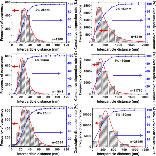
Figure 2.6. Interparticle distance of 25 nm and 150 nm nanoparticles within the matrix for volume fractions of 2%, 4% and 6%. For a color version of this figure, see www.iste.co.uk/bai/nanocomposites.zip
Table 2.1. Diameters, dispersion rates and interparticle distances (TEM)
| Size (nm) | Parameters | 2% | 4% | 6% |
| 15 | Diameter (nm) | 11.1 ± 0.3 | 13.8 ± 0.7 | 11.4 ± 1.2 |
| Dispersion (%) | 35 | 45 | 48 | |
| Interparticle distance (nm) | 37.9 ± 1.7 | 27.7 ± 0.2 | 26.9 ± 0.2 | |
| 25 | Diameter (nm) | 26 ± 0.1 | 22.3 ± 0.1 | 26.5 ± 0.2 |
| Dispersion (%) | 67 | 74 | 65 | |
| Interparticle distance (nm) | 30 ± 0.3 | 24.7 ± 0.16 | 32.7 ± 0.5 | |
| 60 | Diameter (nm) | 65.4 ± 0.5 | 68.2 ± 0.3 | 53 ± 0.9 |
| Dispersion (%) | 73 | 68 | 50 | |
| Interparticle distance (nm) | 47.5 ± 0.1 | 48.5 ± 0.1 | 39.7 ± 1.3 | |
| 150 | Diameter (nm) | 166.2 ± 1.9 | 175.6 ± 1.5 | 171.2 ± 0.8 |
| Dispersion (%) | 74 | 75 | 80 | |
| Interparticle distance (nm) | 411.7 ± 12.9 | 403.2 ± 3.6 | 351.6 ± 0.5 | |
| 500 | Diameter (nm) | 452.1 ± 5.4 | 474.4 ± 9.4 | 389.6 ± 0.6 |
| Dispersion (%) | 75 | 63 | 83 | |
| Interparticle distance (nm) | 1,063.8 ± 47.4 | 825.9 ± 31.2 | 645 ± 20.7 |
2.2. X-ray diffraction
The X-ray diffraction measurements performed in this chapter were performed on the synchrotron 5-DND-CAT sector line at the Center for Nanoscale Materials at the Argonne National Laboratory1. The wavelength of the beam is λ = 0.7293 Å–1. In addition to observations at various angles, the equipment available on this line is capable of monitoring temperature for thermal testing.
The measurements at small and wide angles lead to obtaining distances between:
- – SAXS (small angle X-ray scattering): 0.00239 ≤ q ≤ 0.144 Å–1 (2,630 ≥ d ≥ 44 Å);
- – MAXS (middle angle X-ray scattering): 0.133 ≤ q ≤ 0.826 Å–1 (47.2 ≥ d ≥ 7.61 Å);
- – WAXS (wide angle X-ray scattering): 0.67 ≤ q ≤ 4.5 Å–1 (9.4 ≥ d ≥ 1.4 Å).
The advantage of the synchrotron compared to conventional X-ray diffraction lies in the exposure time of the sample to the beam. Due to its high power, the synchrotron is capable of providing a very short exposure time compared to the equipment we have in the laboratory. In addition to the accumulation of noise that can result from a long exposure to the beam, this can also cause a local heating of the material and thus modify the microstructure. The sample exposure and data acquisition times are, respectively, 0.01 s and 0.012 s. The distance between the sample and the SAXS sensor is 8502.5 mm and that to the WAXS sensor is 200 mm.
2.2.1. SAXS
Small-angle diffraction measurements are used to determine the size of the nanoparticles, aggregates and interparticle distances. For the tests, the samples were placed in an aluminum crucible that served as a support. The tests were performed on the matrix, the nanoparticles, the nanocomposites and the empty crucible (support). The diffraction data obtained at the end of each test are those for the sample and the crucible. To obtain the data from the sample or the nanoparticles contained in the nanocomposites, we made two corrections. We subtracted the crucible and matrix data first and then applied the Porod correction (Porod 1951; Schnablegger and Singh 2013). The Porod correction is a mean used to correct the curve at large q values of the SAXS data. The curve of the diffracted intensity as a function of the inverse of q4 (I vs. 1/q4) is approximated by linear regression at large values of q. The Porod correction consists of subtracting the value of the intercept of this regression from the diffracted intensity. With the corrected data, we proceeded to analyses in different zones, such as the Guinier zone to determine the size of the nanoparticles, the Porod zone for their shape and the Fourier zone for the interparticle distances.
Figure 2.7 shows the Porod analyses of (a) 60 nm nanoparticle powder and the 4%/60 nm nanocomposite and (b) 150 nm nanoparticle powder and the 4%/150 nm nanocomposite. In Figure 2.7(a), the linear regression of the curves at large values of q showed distributions in q–4 and q–3.6, respectively, for the nanoparticles in the silica powder and those in the 4%/60-nm nanocomposite. An evolution of the curve in q–4 is characteristic of perfectly spherical nanoparticles. It thus reveals that the nanoparticles are spherical before being incorporated into the matrix. An evolution of the curve in q–3.6 is characteristic of an intermediate shape between the spherical and flat shapes. Given that the nanoparticles are initially spherical, we deduce that this is the shape of agglomerated nanoparticles. Indeed, in the case of powders, the nanoparticles are isolated from each other and well dispersed, which allows the evolution of the curves at q–4. When the nanoparticles are incorporated into the matrix, chemical bonds are created which, when they are stronger than the nanoparticle–nanoparticle bonds, allow a good nanoparticle distribution within the matrix, but if they are not, they lead to the formation of aggregates. The shape of the aggregates combined with the spherical shape of nanoparticles is responsible for the q–3.6 evolution of the 4%/60 nm intensity curve (Schnablegger and Singh 2013; GmbH AP. SAXS-Data Classification 01-Basics).
In Figure 2.7(b), the linear regression at large values of q is q–4 for the powder and nanocomposites. We thus notice that, unlike 60 nm nanoparticles, 150 nm nanoparticles are well dispersed in the matrix. In this figure, the periodic evolution of the curve is another observation that gives information on the state of the nanoparticle distribution. This evolution is characteristic of monodispersity (Schnablegger and Singh 2013; GmbH AP. SAXS-Data Classification 01-Basics). The Porod analysis was carried out on nanoparticles and nanocomposites, and we noticed that all powdered nanoparticles present a q–4 evolution at large values of q. For nanoparticles smaller than 60 nm in diameter mixed with the matrix, the intensity curve evolves in q–α with α < 4. For nanoparticles of diameter 150 nm and above, we have an evolution in q–4, whether they are mixed with the matrix or not. For the same nanoparticle sizes, we also remarked the periodic evolution of the curves, regardless of the volume fraction. We note that the critical size from which the nanoparticles start to agglomerate is between 60 nm and 150 nm.
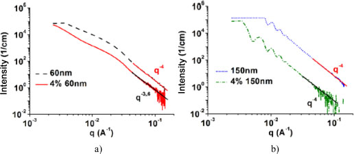
Figure 2.7. Porod analysis of a) 60 nm nanoparticle powders and nanoparticles contained in the 4%/60 nm nanocomposite; b) 150 nm nanoparticle powders and nanoparticles contained in the 4%/150 nm nanocomposite. For a color version of this figure, see www.iste.co.uk/bai/nanocomposites.zip
Figure 2.8 shows the Guinier analysis of 60 nm nanoparticles in powder and in the 4% nanocomposite. This analysis makes it possible to determine the average radius of the nanoparticles. It consists of achieving a linear regression at the very low values of the natural logarithm curve of the intensity with respect to the square of the diffusion vector (Ln(I) vs. q2). Guinier has shown that at very low values of q, the size of nanoparticles can be determined (Guinier and Fournet 1956; Glatter and Kratky 1982). By comparing the linear regression of the nanoparticle powder to that of the nanocomposite, one can note that the regression of the nanocomposite curve is not linear. The nanocomposite has a nonlinear evolution at low values of q, which is characteristic of the presence of aggregates, as observed in Figure 2.7(a). The linear regression is effective when the nanoparticles are well dispersed; otherwise, the analysis can lead to errors, namely by giving the average radius of the set of nanoparticles and aggregates and not the respective radii of the nanoparticles and aggregates. As our materials contain aggregates mainly at low nanoparticle sizes, the Guinier analysis was not conclusive.
We then focused on the deconvolution technique. The first step is to apply the Lorentz correction. This consists of multiplying the diffracted intensity by q2 and results in bringing out the positions of the peaks, which are sometimes difficult to distinguish. The positions of the peaks, which are determined at maximum intensities, can be used to determine characteristic lengths by the Bragg law. The application of this correction has no effect on the SAXS curves of a randomly oriented crystal or material with well-defined peaks, and the effect is to shift the peak positions slightly to higher values (Dlugosz et al. 1976; Cser 2001).
The use of the Lorentz correction is difficult in the case of a multiphase material. Indeed, the diffusion curve of a multiphase material is the sum of the diffusion intensities of the different phases and the interactions between these phases. For example, in a periodic material there are characteristic lengths that, on the SAXS curve, produce a peak or a series of peaks whose exact positions are determined based on the Lorentz correction. If nanoparticles can also be found in the same material, their characteristic scatterings will be combined with those of the characteristic lengths. In this case, with the Lorentz correction, the positions of the peaks with maximum intensities no longer correspond to the characteristic lengths of the periodic phase or to the nanoparticles. A deconvolution of the general curve must therefore be done to separate the different scattering curves and determine the positions of the different peaks. In the case where the Guinier analysis was not conclusive, the deconvolution technique is preferred in order to separate the contributions of the different sizes present in the material.
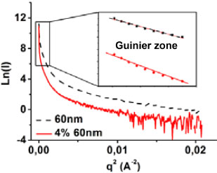
Figure 2.8. Guinier analysis for powders of 60 nm nanoparticles and nanoparticles contained in the 4%/60 nm nanocomposite. For a color version of this figure, see www.iste.co.uk/bai/nanocomposites.zip
Figure 2.9 shows the deconvolved curves of the diffracted intensity as a function of the scattering vector of the 4%/15 nm and 4%/60 nm nanocomposites. The solid curves are the experimental curves obtained after the Lorentz correction, and the dashed and mixed curves are those obtained after deconvolution. The dashed curves represent the contributions of the shape factors while the mixed curves are that of the structure factor. The shape factor gives information on the size and areas of the nanoparticles, while the structure factor gives information on the interparticle distances (GmbH AP. SAXS-Data Classification 01-Basics). The peaks of the dashed lines give the sizes of the nanoparticles with the Bragg law and the position of the peak of the dot-dash line curve gives an approximate value of the interparticle distance. The ratio of the area under a form factor curve to the total area is taken as the distribution rate of nanoparticles of corresponding size at this curve. Deconvolution of the 4%/15 nm nanocomposite curve (Figure 2.9(a)) yielded three different sizes of nanoparticles with corresponding ratios. In the case of the 4%/60 nm nanocomposite, two sizes were obtained (Figure 2.9(b)). In the 4%/15 nm nanocomposite, there were 21% nanoparticles with a diameter of 16 ± 1 nm, 60% with 31 ± 3 nm and 19% with 97 ± 2 nm. The 4%/60 nm nanocomposite contained 67% of 63 ± 4 nm diameter nanoparticles and 37% of 123 ±6 nm diameter nanoparticles. In the two nanocomposites presented, a rate of aggregation can be observed that increases with the decrease in nanoparticle size. By decreasing the size of the nanoparticles, the surface tension increases and the nanoparticles are more attracted to each other and mix less efficiently with the matrix. The position of the peak of the dot-dash line curve gives the average distance of the centers of mass of a nanoparticle and its nearest neighbor. To determine the interparticle distance, the sum of the radii of the two nanoparticles in question must be subtracted from the average distance. In the case of our materials, the variability of the size of nanoparticles and aggregates makes this task more complicated. In order to get an interparticle distance, we subtracted the diameter of the nanoparticles with the highest proportion from the average distance.
Indeed, the higher the proportion of a nanoparticle size, the greater the probability of having a nanoparticle of that size as a nearest neighbor. For example, in the case of the 4%/60 nm nanocomposite, we subtracted 63 nm from the average distance, which is the most represented nanoparticle size in the material (67%). In cases where the nanoparticles are well dispersed, such as for nanoparticles of diameters 150 nm and 500 nm, only one nanoparticle size was obtained and the determination of the interparticle distance is easier. The determination of nanoparticle sizes and interparticle distances was performed for the four volume fractions and five sizes studied, and the results are reported in Table 2.2.
In Table 2.2, we can see that, for small nanoparticle sizes, the size of aggregates increases with the volume fraction and that, unlike what might be expected, their proportion decreases in favor of intermediate-sized nanoparticles (doublet or triplet of nanoparticles). Indeed, by increasing the volume fraction, not only does the probability of having many more aggregates increase but so does that of having many more isolated nanoparticles. Moreover, the nanoparticles agglomerating into a large nanoparticle have a reduced surface tension and, under the effect of the matrix interactions, burst and form aggregates of intermediate size, as can be seen for the 6% and 8% volume fractions.
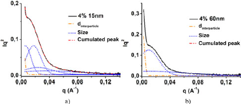
Figure 2.9. Decomposition of the intensity curves: a) from 4%/15 nm and b) 4%/60 nm after Lorentz correction. For a color version of this figure, see www.iste.co.uk/bai/nanocomposites.zip
Table 2.2. Diameters, dispersion rates and interparticle distances (SAXS)
| Fraction vol (%) | Theoretical diameter (nm) | Measured diameters (nm) | Proportion (%) | dinterparticle (nm) |
| S(q) | ||||
| 2% | 15 | 16± 1 (11.1)* | 26 (35)* | 65 |
| 23 ±3 | 15 | |||
| 73 ±2 | 59 | |||
| 25 | 28 ± 4 (26)* | 43 (67)* | 61 | |
| 86 ±1 | 57 | |||
| 60 | 59 ± 2 (65.4)* | 30 (73)* | 79 | |
| 111±4 | 70 | |||
| 150 | 179 ±2 (166.2)* | ≈100 (74)* | – | |
| 500 | 492 ±5 (452.1)* | ≈100 (75)* | – | |
| 4% | 15 | 16 ± 1 (13.8)* | 21 (45)* | 86 |
| 31 ±3 | 60 | |||
| 97 ±2 | 19 | |||
| 25 | 26 ± 1 (22.3)* | 53 (74)* | 152 | |
| 84 ±4 | 47 | |||
| 60 | 63 ± 4 (68.2)* | 67 (68)* | 113 | |
| 123 ±6 | 33 | |||
| 150 | 179 ±2 (175.6)* | ≈100 (75)* | – | |
| 500 | 492 ± 5 (474.4)* | ≈100 (63)* | – | |
| 6% | 15 | 16 ± 1 (11.4)* | 25 (48)* | – |
| 27 ±4 | 36 | |||
| 46 ±1 | 22 | |||
| 124 ±7 | 17 | |||
| 25 | 28 ± 4 (26.5)* | 45 (65)* | 41 | |
| 57 ±2 | 55 | |||
| 60 | 61 ±2 (53)* | 64 (50)* | 32 | |
| 124 ±5 | 36 | |||
| 150 | 179 ±2 (171.2)* | ≈100 (80)* | – | |
| 500 | 492 ± 5 (389.6)* | ≈100 (83)* | – | |
| 8% | 15 | 17 ± 1* | 31* | 114 |
| 30 ±3 | 33 | |||
| 48 ±2 | 29 | |||
| 82 ±5 | 7 | |||
| 25 | 28 ±2* | 66* | 101 | |
| 42 ±4 | 16 | |||
| 95 ±3 | 18 | |||
| 60 | 58± 1* | 31* | 105 | |
| 109 ±3 | 69 | |||
| 150 | 179 ±2* | ≈100* | – | |
| 500 | 492 ±5* | ≈100* | – |
* Diameters and proportions measured by TEM.
2.2.2. WAXS
Wide-angle diffraction tests are performed under the same conditions as those performed at small angles. The only difference is the position of the sensor, which is 200 mm from the sample. While small-angle diffraction helps to determine nanoparticle sizes and interparticle distances, wide-angle diffraction allows intermolecular or intramolecular distances to be determined. The sensor used at wide angles makes it possible to determine distances between 1.4 and 9.4 Å. The values of inter- and intramolecular distances in polymers range between 2 and 7 Å. The range covered by the X-ray wide-angle diffraction will thus enable us to determine these distances and follow their evolution according to the size of the nanoparticles.
Prior to any analysis, the raw data of the matrix, nanoparticles and nanocomposites are corrected and processed. The correction consists of subtracting the signal of the crucible from each signal. Figure 2.10 illustrates the wide-angle diffraction curves of PMMA, the 60 nm diameter silica nanoparticles and the 4%/60 nm nanocomposite. The silica curve shows a broad peak around q = 1.555 Å–1. The broad peaks are characteristic of amorphous materials and the silica diffraction curve confirms the choice of the silica structure. On the diffraction curve of the matrix three broad peaks can be observed, which also attest to the amorphous structure of the matrix. The same peaks are also observed for the 4%/60 nm nanocomposite. In addition to the matrix peaks, one can also note, although not visible, the silica nanoparticle peak on the 4%/60 nm nanocomposite curve. Furthermore, compared to the PMMA curve, we observe a slight variation in the slope of the 4%/60 nm curve around the position of the silica peak. This variation is due to the silica signal that is included in the global signal of the nanocomposite. This signal, when well determined, is used for the calculation of the mass fraction of nanoparticles present in the material. The mass fraction is obtained by the ratio of the area under the curve of the nanoparticles to the total area of the nanocomposite.
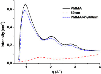
Figure 2.10. Diffraction PMMA, 60 nm nanoparticles and 4%/60 nm nanocomposite curves. For a color version of this figure, see www.iste.co.uk/bai/nanocomposites.zip
On the one hand, these observations confirm that the addition of nanosized fillers did not change the structure of the matrix (amorphous) and, on the other hand, validate the choice of our materials. It can thus be deduced that any variation of the characteristic lengths of the matrix in the presence of nanoparticles will only be due to the size of the latter.
To get the characteristic lengths in the matrix and nanocomposites, we applied a method that consists of deconvoluting the corrected experimental signal into Gaussians (Wang et al. 2008; Gelineau 2015). Each Gaussian corresponds to an intramolecular or intermolecular distance. The deconvolution was done with a baseline connecting the two ends of the signal (Wang et al. 2008; Gelineau 2015). Figure 2.11 represents the deconvoluted signal of the matrix. The matrix curve shows three peaks. The deconvolution of this curve could be done with three Gaussians, however, the asymmetry of the first peak may be the result of the superposition of two peaks. Further works in the literature have shown that the wide-angle diffraction curve of PMMA consists of four peaks (Lovell and Windle 1981). The deconvolution of the curve is done with four Gaussians. Peak 1 corresponds to the intermolecular distance and the other three correspond to intramolecular distances. As a matter of fact, the position of peak 1 (q1 = 0.916 Å–1) is used to determine the distance between the chains of the matrix and those of peaks 2 (q2 = 1.125 Å–1), 3 (q3 = 2.05 Å–1) and 4 (q4 = 2.854 Å–1) to determine the distances between the different groups which constitute the matrix chains. In their work, Lovell and Windle (1981) attributed the characteristic length corresponding to the position of peak 2 to the distance between two consecutive planes of carbonyl groups. Since the PMMA utilized in this research is atactic, similar to the one whose conformation is proposed by Lovell and Windle (1981), the plane defined by the carboxyl groups is the one which passes through two groups located on each side of the carbon chain. The distance d3 corresponds to the distance between two planes of the methyl groups and d4 is the distance between backbone carbon atoms (Lovell and Windle 1981). Using Bragg’s law, we obtain d1 = 6.86 Å, d2 = 5.59 Å, d3 = 3.06 Å and d4 = 2.2 Å. These distances are similar to those found in the literature.
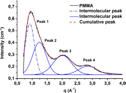
Figure 2.11. Deconvolution of the of PMMA wide-angle diffraction. For a color version of this figure, see www.iste.co.uk/bai/nanocomposites.zip
After determining the characteristic lengths existing in the matrix, we performed a comparison of the matrix diffraction curve with those of these nanocomposites as a function of size. In order to compare curves that are at the same scale, we normalized each diffraction curve by its maximum intensity. Figure 2.12 shows the PMMA diffraction curves and its 4% nanocomposites for the different sizes at a temperature of 30°C. Only the areas concerning the first three peaks of the matrix are shown because no significant variation was observed for the position of peak 4. A difference in the shape of the curves is observed in the area corresponding to the positions of peak 2 and the silica peak that we will name peak 5. The position of peak 3 does not seem to change. This difference in shape is reflected by a swelling of the curve. This swelling becomes more and more important with the decrease in the size of the nanoparticles. It may be due to an excessive proportion of nanoparticles in the matrix or to a shift in the positions of peaks 2 and/or 3 toward large values of q. Since the volume fraction of the nanoparticles is constant, it is deduced that this swelling is due to a shift in the positions of peaks 2 and/or 3 toward large values of q. This shift is all the more important as the size of the nanoparticles decreases. The more the position of the peaks is shifted toward higher values of q, the larger the corresponding values by the Bragg law. We also note that the position of the peak with maximum intensity, that corresponds to that of peak 1, varies very little with the size of the nanoparticles. This study shows that at the temperature of 30°C (in the glassy state), the size effect of the nanoparticles on the characteristic lengths of the matrix results in a shift in the position of the peaks corresponding to the distances d1 and/or d2 and, more particularly, of d2. The size effect leads to a decrease in the interparticle distance and the intramolecular distance between the carbonyl planes.
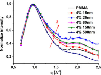
Figure 2.12. Comparison of the wide-angle diffraction curves of PMMA and its nanocomposites loaded to 4% and different sizes. For a color version of this figure, see www.iste.co.uk/bai/nanocomposites.zip
In order to achieve a quantitative study of the size effect on the micro-structural parameters of the matrix, the diffraction curves of the nanocomposites were deconvolved and the corresponding distances to the peak positions are compared. Considering the high sensitivity of d2 to the variation of the nanoparticle size compared to the sensitivity of d1, we compared the distance d2 of the matrix to that of the nanocomposites. Figure 2.13 presents the evolutions of the d2 distances of the nanocomposites as a function of the nanoparticle size for the four volume fractions. The d2 distances of the nanocomposites are normalized by that of the matrix (d2 = 5.59 Å). It is generally observed that the intramolecular distance separating the carbonyl planes in the nanocomposites is smaller than that present in the matrix except for 4%/500 nm, 2%/150 nm and 2%/500 nm. At constant volume fraction, d2 decreases with decreasing nanoparticle size independently of the volume fraction. The nanoparticles with their nanometric dimensions mix with the matrix chains. The nanometric dimensions of the nanoparticles seem to have an effect on the conformation of the matrix chains. In response to the presence of nanoparticles in the matrix, the chains reorganize themselves by changing their configuration.
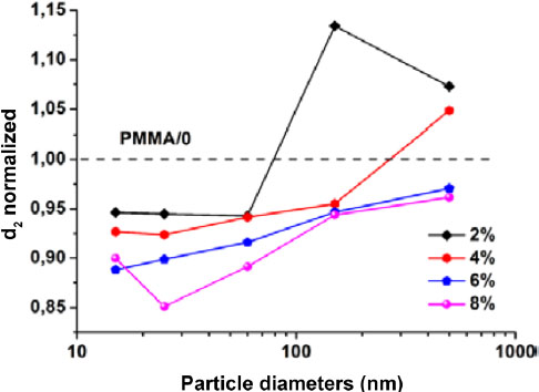
Figure 2.13. Evolution of the normalized intramolecular distance (d2) of the matrix in nanocomposites as a function of nanoparticle size and volume fraction (d2 PMMA = 5.59 Å). For a color version of this figure, see www.iste.co.uk/bai/nanocomposites.zip
X-ray diffraction was used to determine the characteristic lengths of the nanoparticles (SAXS) and the matrix (WAXS). With the SAXS observations, the size of the nanoparticles and aggregates, as well as their rate, were determined with much more precision. The TEM also led to determining these parameters but it was less easy to grasp the size of the aggregates and their rate at low nanoparticle sizes. The WAXS observations made characteristic lengths that are not visible with TEM accessible. Thus, they showed that the inter- and intramolecular bonds are dependent on the size of the nanoparticles. The decrease in nanoparticle size is accompanied by a decrease in the length of these bonds.
2.3. Conclusion
The study of the effect of filler size on the properties of nanocomposites requires a good choice of matrix, fillers, processing and also a fine microstructure characterization. The main criterion, which is to have the size of the fillers as the only variable factor among the parameters that can modify the microstructure, led to the choices of PMMA for the matrix and silica nanoparticles for the fillers. These choices have allowed us to overcome any crystallization of the matrix in the presence of the fillers, as shown by the diffraction curves of nanocomposites.
The different observation techniques (TEM and SAXS) revealed a variation of the characteristic lengths according to the size of the nanoparticles and at all scales. At the microscopic scale, direct observations showed that the choice of the implementation process allowed for a good distribution of the nanoparticles in the matrix but was not sufficient to avoid the aggregation of small nanoparticle sizes. This aggregation, even if it does happen, is limited to the formation of nanoparticle doublets or triplets, which is still acceptable given the strong attractiveness that exists between silica nanoparticles. The interparticle distances also decrease with decreasing nanoparticle size. At the molecular scale (WAXS), the size of the nanoparticles acts on the interchain bonds by confining the chains between the nanoparticles. This results in a decrease of these bonds with the decrease in the nanoparticle sizes. The decrease in these distances will lead to a reduction of chain mobility. As the properties of the polymers are intrinsically linked to chain mobility, this reduction in the distance could generate a modification of the properties of the matrix.
Morphological characterization has made it possible to identify parameters from the microstructure up to the molecular scale (particle and aggregate sizes, interparticle and interchain distances). In Chapter 3, we will focus on the impact of size on the physicochemical and mechanical properties and we will try to link the identified parameters to the measured properties.
2.4. References
Banfield, J.F. and Zhang, H. (2001). Nanoparticles in the environment. Rev. Mineral Geochemistry, 44(1), 1–58.
Cheng, B., Kng, J., Luo, J., Dong, Y. (1993). Relation of structure stability and Debye temperature to crystal size of nanometer sized TiO_2 powders. Chin. J. Mater. Res., 7(3), 240–243.
Cser, F. (2001). About the Lorentz correction used in the interpretation of small angle X-ray scattering data of semicrystalline polymers. J. Appl. Polym. Sci., 80, 2300–2308.
Dlugosz, J., Fraser, G.V., Grubb, D., Keller, A., Odell, J.A., Goggin, P.L. (1976). Study of crystallization and isothermal thickening in polyethylene using SAXD, low frequency Raman spectroscopy and electron microscopy. Polymer, 17(6), 471–480.
Gelineau, P. (2015). Caractérisation morphologique et homogénéisation élastique et visco-élastique de polymère. PhD Thesis, Université de technologie de Compiégne.
Glatter, O. and Kratky, O. (1982). Small Angle X-ray Scattering. Academic Press, London.
González, I., Eguiazábal, J.I., Nazábal, J. (2008). Effects of the processing sequence and critical interparticle distance in PA6-clay/mSEBS nanocomposites. Eur. Polym. J., 44(2), 287–299.
Guinier, A. and Fournet, G. (1956). Small angle scattering of X-rays. J. Polym. Sci., 19, 594–594.
Kavesh, S. and Schultz, J.M. (1970). Lamellar and interlamellar structure in melt-crystallized polyethylene I. Degree of crystallinity, atomic positions, particle size, and lattice disorder of the first and second kinds. J. Polym. Sci., Part A-2: Polym. Phys., 8(2), 243–276.
Lovell, R. and Windle, A.H. (1981). Determination of the local conformation of PMMA from wide-angle X-ray scattering. Polymer, 22(2), 175–184.
Porod, G. (1951). Die Röntgenkleinwinkelstreuung von dichtgepackten kolloiden Systemen. Kolloid-Z, 124, 83–114.
Rasband, W. (2012). ImageJ software release 1.48v [Online]. Available at: http://imagej.nih.gov/ij.
Schnablegger, H. and Singh, Y. (2013). The SAXS guide: Getting acquainted with the principles. Guide, Anton Paar GmbH, Austria, 37–84.
Shin, H., Yang, S., Choi, J., Chang, S., Cho, M. (2015). Effect of interphase percolation on mechanical behavior of nanoparticle-reinforced polymer nanocomposite with filler agglomeration: A multiscale approach. Chem. Phys. Lett., 635, 80–85.
Tessema, A., Zhao, D., Moll, J., Xu, S., Yang, R., Li, C., Kumar, S.K., Kidane, A. (2017). Effect of filler loading, geometry, dispersion and temperature on thermal conductivity of polymer nanocomposites. Polym. Test., 57, 101–106.
Wang, W., Murthy, N.S., Chae, H.G., Kumar, S. (2008). Structural changes during deformation in carbon nanotube-reinforced polyacrylonitrile fibers. Polymer, 49, 2133–2145.
- 1 Available at: www.anl.gov/cnm.