Rolling Buffers

A rolling buffer is a location in memory where data is dumped cyclically: information is dropped linearly, and when the buffer is filled up, data is dumped at the beginning of the buffer, and the process repeats. Example 3-1 gives an example of using a rolling buffer with tcpdump: in this example, the process writes approximately 128 MB to disk (specified by the -C switch), and then rotates to a new file. After 32 files are filled (specified by the -W switch), the process restarts.

$ tcpdump -i en1 -s 0 -w result -C 128 -W 32

Rolling buffers implement a time horizon on traffic analysis: data is available only as long as it’s in the buffer. For that reason, working with smaller file sizes is recommended, because when you find something aberrant, it needs to be pulled out of the buffers quickly. If you want a more controlled relationship for the total time recorded in a buffer, you can use the -G switch to specify that a file should be dumped at a fixed interval (specified by -G) rather than a fixed size.

Limiting the Data Captured from Each Packet

An alternative to capturing the complete packet is to capture a limited subset of the payload, controlled in tcpdump by the snaplen (-s) argument. Snaplen constrains packets to the frame size specified in the argument. If you specify a frame size of at least 68 bytes, you will record the TCP or UDP headers.¹ That said, this solution is a poor alternative to NetFlow, which is discussed later in this chapter.

Filtering Specific Types of Packets

An alternative to filtering at the switch is to filter after collecting the traffic at the spanning port. With tcpdump and other tools, this can be easily done using BPF. BPF allows an operator to specify arbitrarily complex filters, and consequently the possibilities are fairly extensive. Some useful options are described in this section, along with examples. Figure 3-1 provides a breakdown of the headers for Ethernet frames, IP, UDP, ICMP, and TCP.

As we walk through the major fields, I’ll identify BPF macros that describe and can be used to filter on these fields. On most Unix-style systems, the pcap-filter manpage provides a summary of BPF syntax. Available commands are also summarized in the FreeBSD manpage for BPF.

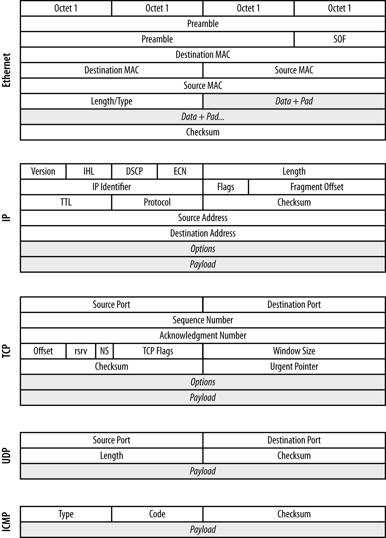
Figure 3-1. Frame and packet formats for Ethernet, IP, TCP, UDP, and ICMP

In an Ethernet frame, the most critical fields are the two MAC addresses: destination MAC and source MAC. These 48-bit fields are used to identify the hardware addresses of the interfaces that sent and will receive the traffic. MAC addresses are restricted to a single collision domain, and will be modified as a packet traverses multiple networks (see Figure 2-5 for an example). MAC addresses are accessed using the ether src and ether dst predicates in BPF.²

Within an IP header, the fields you are usually most interested in are the IP addresses, the length, the TTL, and the protocol. The IP identifier, flags, and fragment offset are used for attacks involving packet reassembly—however, they are also largely a historical artifact from before Ethernet was a nearly universal transport protocol. You can get access to the IP addresses using the src host and dst host predicates, which also allow filtering on netmasks.

To filter on protocols, use the ip proto predicate. BPF also provides a variety of protocol-specific predicates, such as tcp, udp, and icmp. Packet length can be filtered using the less and greater predicates, while filtering on the TTL requires more advanced bit manipulation, which is discussed later.

The following snippet filters out all traffic except that coming within this block (hosts with the netmask /24):

host$ tcpdump -i en1 -s 0 -w result src net 192.168.2.0/24

Example 3-2 demonstrates filtering with tcpdump.

# Filtering out everything but internal traffic
host$ tcpdump -i en1 -s 0 -w result src net 192.168.2.0/24 && dst net 
      192.168.0.0/16
# Filtering out everything but web traffic, identified by port
host$ tcpdump -i en1 -s 0 -w result ((src port 80 || src port 443) && 
      (src net 192.168.2.0))

In TCP, the port number and flags are the most critical for investigation, analysis, and control. TCP flags are used to maintain the TCP state machine, while the port numbers are used to distinguish sessions and for service identification. Port numbers can be filtered using the src port and dst port switches, as well as the src portrange and dst portrange switches, which filter across a range of port values. BPF supports a variety of predicates for TCP flags, including tcp-fin, tcp-syn, tcp-rst, tcp-push, tcp-ack, and tcp-urg.

As with TCP, the UDP port numbers are the most important information for analyzing and controlling the traffic. They are accessible using the same port and portrange switches as TCP.

Because ICMP is the internet’s error message–passing protocol, ICMP messages tend to contain extremely rich data. The ICMP type and code are the most useful for analysis because they define the syntax for whatever payload (if any) follows. BPF provides a variety of type- and code-specific filters, including icmp-echoreply, icmp-unreach, icmp-tstamp, and icmp-redirect.

What If It’s Not Ethernet?

For the sake of brevity, this book focuses exclusively on IP over Ethernet, but you may well encounter a number of other transport and data protocols. The majority of these protocols are highly specialized and may require additional capture software besides the tools built on libpcap. A few of the more common ones are:

ATM

Asynchronous Transfer Mode, the great IP slayer of the ’90s. ATM is now largely used for ISDN and PSTN transport, and some legacy installations.

Fibre Channel

Primarily used for high-speed storage, Fibre Channel is the backbone for a variety of SAN implementations.

CAN

Controller area network. Primarily associated with embedded systems such as vehicular networks, CAN is a bus protocol used to send messages in small isolated networks.

These protocols are scratching the surface. In particular, if you’re dealing with industrial control systems, you can expect to find a maze of proprietary protocols. When dealing with industrial systems, find their manuals first—it’s likely to be the only way you can do anything akin to packet capture.

Any form of filtering imposes performance costs. Implementing a spanning port on a switch or a router sacrifices performance that the switch or router could be using for traffic. The more complicated a filter is, the more overhead is added by the filtering software. At nontrivial bandwidths, this will be a problem.

NetFlow v5 Formats and Fields

NetFlow v5 is the earliest common NetFlow standard, and it’s worth covering the values in its fields before discussing alternatives. NetFlow v5’s fields (listed in Table 3-1) fall into three broad categories: fields copied straight from IP packets, fields summarizing the results of IP packets, and fields related to routing.

The srcaddr, dstaddr, srcport, dstport, prot, and tos fields of a NetFlow record are copied directly from the corresponding fields in IP packets. Flows are generated for every protocol in the IP suite, however, and that means that the srcport and dstport fields, which strictly speaking are TCP/UDP phenomena, don’t necessarily always mean something. In the case of ICMP, NetFlow records the type and code in the dstport field. In the case of other protocols, the value is meaningless; depending on the collection system you may end up with a previously allocated value, zeros, or other data.

The packets, dOctets, first, last, and tcp_flags fields all summarize traffic from one or more packets. packets and dOctets are simple totals, with the caveat that the dOctets value is the layer 3 total of octets, meaning that IP and protocol headers are added in (e.g., a one-packet TCP flow with no payload will be recorded as 40 bytes, and a one-packet UDP flow with no payload as 28 bytes). The first and last values are, respectively, the first and last times observed for a packet in the flow.

tcp_flags is a special case. In NetFlow v5, the tcp_flags field consists of an OR of all the flags that appear in the flow. In well-formed flows, this means that the SYN, FIN, and ACK flags will always be high for any valid TCP session.

The final set of fields—nexthop, input, output, src_as, dst_as, src_mask, and dst_mask—are all routing-related. These values can be collected only at a router.

NetFlow Generation and Collection

NetFlow records are generated directly by networking hardware appliances (e.g., a router or a switch), or by using software to convert packets into flows. Each approach has different trade-offs.

Appliance-based generation means using whatever NetFlow facility is offered by the hardware manufacturer. Different manufacturers use similar-sounding but different names than Cisco, such as JFlow by Juniper Networks and NetStream by Huawei. Because NetFlow is offered by so many different manufacturers with a variety of different rules, it’s impossible to provide a technical discussion about the necessary configurations in the space provided by this book. However, the following rules of thumb are worth noting:

• NetFlow generation can cause performance problems on routers, especially older models. Different companies address this problem in different ways, ranging from reducing the priority of the process (and dropping records) to offloading the NetFlow generation task to optional (and expensive) hardware.

• Most NetFlow configurations default to some form of sampling in order to reduce the performance load. For security analysis, NetFlow should be configured to provide unsampled records.

• Many NetFlow configurations offer a number of aggregation and reporting formats. You should collect raw NetFlow, not aggregations.

The alternative to router-based collection is to use an application that generates NetFlow from pcap data, such as CERT’s Yet Another Flowmeter (YAF) tool, softflowd, or the extensive flow monitoring tools provided by QoSient’s Argus tool. These applications take pcap as files or directly off a network interface and aggregate the packets as flows. These sensors lack a router’s vantage, but are able to devote more processing resources to analyzing the packets and can produce richer NetFlow output, incorporating features such as deep packet inspection.

Classifying IDSs

We can divide IDSs along two primary axes: the IDS domain, and the decision-making process. On the first axis, IDSs are broken into network-based IDSs (NIDSs) and host-based IDS (HIDSs). On the second axis, IDSs are split between signature-based systems and anomaly-based systems. Relating these terms back to our earlier taxonomy, NIDSs operate in the network domain, HIDSs in the host domain. The classic IDS is an event sensor; there are controller systems, IPSs, which will control traffic in response to aberrant phenomena. This section focuses on NIDSs—network-domain event-action sensors.

A NIDS is effectively any IDS that begins with pcap data. For open source IDSs, this includes systems such as Snort, Bro, and Suricata. NIDSs operate under the constraints discussed for network sensors in Chapter 2, such as the need to receive traffic through port mirroring or direct connection to the network and an inability to read encrypted traffic.

For the purposes of simplicity, in this section we will treat all IDSs as signature-based. A signature-based system uses a set of rules that are derived independently from the target in order to identify malicious behavior.

IDS as Classifier

All IDS are applied exercises in classification, a standard problem in AI and statistics. A classifier is a process that takes in input data and classifies the data into one of at least two categories. In the case of IDS, the categories are usually “attack” and “normal.”

Signature and anomaly-based IDSs view attacks in fundamentally different ways, and this impacts the types of errors they make. A signature-based IDS is calibrated to look for specific weird behaviors such as malware signatures or unusual login attempts. Anomaly-based IDSs are trained on normal behavior and then look for anything that steps outside the norm. Signature-based IDSs have high false negative rates, meaning that they miss a lot of attacks. Anomaly-based IDSs have high false positive rates, which means that they consider a lot of perfectly normal activity to be an attack.

IDSs are generally binary classifiers, meaning that they break data into two categories. Binary classifiers have two failure modes:

False positives

Also called a Type I error, this occurs when something that doesn’t have the property you’re searching for is classified as having the property—for instance, when email from the president of your company informing you about a promotion is classified as spam.

False negatives

Also called a Type II error, this occurs when something that has the property you’re searching for is classified as not having the property. This happens, for instance, when spam mail appears in your inbox.

Sensitivity refers to the percentage of positive classifications that are correct, and specificity refers to the percentage of negative classifications that are correct. A perfect detection has perfect sensitivity and specificity. In the worst case, neither rate is above 50%: the same as flipping a coin.

Most systems require some degree of trade-off; generally, increasing the sensitivity means also accepting a lower specificity. A reduction in false negatives will be accompanied by an increase in false positives, and vice versa.

To describe this trade-off, we can use a visualization called a receiver operating characteristic (ROC) curve (discussed in more depth in Chapter 11). A ROC curve plots the specificity against the false positive rates, using a third characteristic (the operating characteristic) as a control. Figure 3-2 shows an example of a ROC curve.

In this case, the operating characteristic is the number of packets in a session and is shown on the horizontal lines in the plot. At this site, HTTP traffic (falling at the very left edge) has a good ratio of true to false positives, whereas SMTP is harder to classify correctly, and FTP even harder.

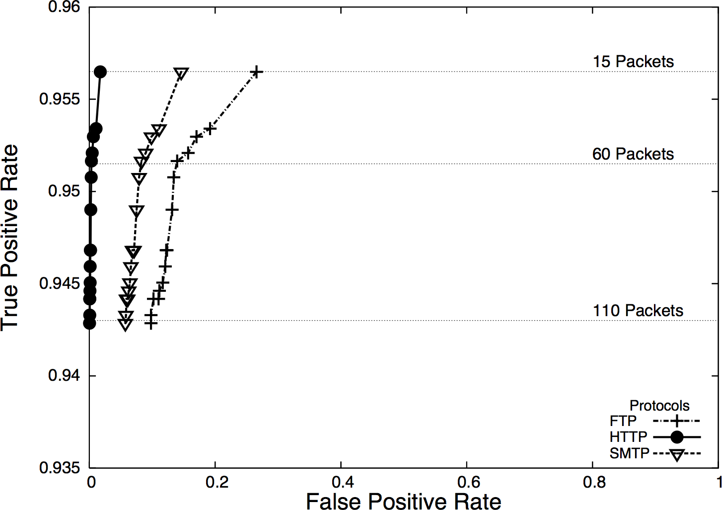
Figure 3-2. ROC curve showing packet size of messages sent for BitTorrent detection

Now, let’s ask a question. Suppose we have an ROC curve and we calibrate a detector so it has a 99% true positive rate and a 1% false positive rate. We receive an alert. What is the probability that the alert is a true positive? It isn’t 99%; the true positive rate is the probability that if an attack took place, the IDS would raise an alarm.

Let’s define a test as the process that an IDS uses to make a judgment call about data. For example, a test might consist of collecting 30 seconds’ worth of network traffic and comparing it against a predicted volume, or examining the first two packets of a session for a suspicious string.

Now assume that the probability of an actual attack taking place during a test is 0.01%. This means that out of every 10,000 tests the IDS conducts, one of them will be an attack. So out of every 10,000 tests, we raise one alarm due to an attack—after all, we have a 99% true positive rate. However, the false positive rate is 1%, which means that 1% of the tests raise an alarm even though nothing happened. This means that for 10,000 tests, we can expect roughly 101 alarms: 100 false positives and 1 true positive, meaning that the probability that an alarm is raised because of an attack is 1/101 or slightly less than 1%.

This base-rate fallacy explains why doctors don’t run every test on every patient. When the probability of an actual attack is remote, the false positives will easily overwhelm the true positives. This problem is exacerbated because nobody in their right mind trusts an IDS to do the job alone.

Consider the data flow in Figure 3-3, which is a simple representation of how an IDS is normally used in defense.

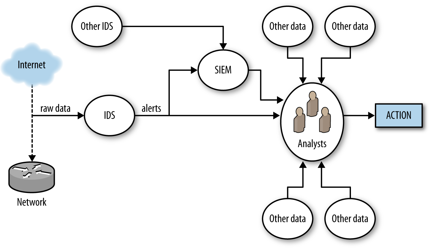
Figure 3-3. Simple detection workflow

Figure 3-3 breaks alert processing into three steps: IDS receives data, raises an alert, and that alert is then passed to analysts either directly or through a security information and event manager (SIEM) console.

Once an IDS generates an alert, that alert must be forwarded to an analyst for further action. Analysts begin by examining it and figuring out what it means. This may be a relatively simple process, but often it becomes wider-ranging and may involve a number of queries. Simple queries will include looking at the geolocation, ownership, and past history of the address the attack originates from (see Chapter 10), by examining the payload of the event using tcpdump or Wireshark. With more complex attacks, analysts will have to reach out to Google, news, blogs, and message boards to identify similar attacks or real-world events precipitating the attack.

With the exception of IPSs, which work on very crude and obvious attacks (such as DDoS attacks), there is always an interim analytical step between alert and action. At this point, analysts have to determine if the alert is a threat, if the threat is relevant to them, and whether or not there’s anything they can do about it. This is a nontrivial problem. Consider the following scenarios:

• The IDS reports that an attacker is exploiting a particular Internet Information Services (IIS) vulnerability. Are there any IIS servers on the network? Have they been patched so they’re not subject to the exploit? Is there evidence from other sources that the attacker succeeded?

• The IDS reports that an attacker is scanning the network. Can we stop the scan? Should we bother given that there are another hundred scans going on right now?

• The IDS reports that a host is systematically picking through a web server and copying every file. Is the host a Google spider, and would stopping it mean that our company’s primary website would no longer be visible on Google?

Note that these are not actually failures on the part of detection. The first two scenarios represent actual potential threats, but those threats may not matter, and that decision can only be made through a combination of context and policy decisions.

Verifying alerts takes time. An analyst might be able to seriously process approximately one alert an hour, and complex events will take days to investigate. Consider how that time is spent given the false positive rates discussed earlier.

Enhancing IDS Detection

Improving an IDS as a classifier involves reducing the false positive and false negative rates. This is generally best done by reducing the scope of the traffic the IDS examines. In the same way that a doctor doesn’t run a test until he has a symptom to work with, we try to run the IDS only when we have an initial suspicion that something odd is going on. A number of different mechanisms are available based on whether you’re using a signature- or an anomaly-based IDS.

One mechanism common to both signature- and anomaly-based IDSs is using inventory to create whitelists. Pure whitelists, meaning that you implicitly trust all traffic from a host, are always a risk. I don’t recommend simply whitelisting a host and never checking it. A better approach, and one that is going to appear in various forms throughout this discussion, is to use whitelisting as a guide for less or more extensive instrumentation.

For example, I create an inventory of all the web servers on my network. A host that is not a web server is suspicious if I see it serving HTTP traffic. In that case, I want to capture a representative cut of traffic and figure out why it’s now a web server. At the same time, for actual web servers, I will use my standard signatures.

In signature-based IDSs, the signature base can usually be refined so that the rule triggers only for specific protocols or in tandem with other indicators. For example, a rule to detect the payload string “herbal supplement” on port 25 will track spam emails with that title, but also internal mail containing comments such as “we’re getting a lot of herbal supplement spam lately.” Reducing the false positive rate in this case involves adding more constraints to the match, such as tracking only mail from outside the network (filtering on addresses). By refining the rule to use more selective expressions, an operator can reduce the false positive rate.

Configuring Snort

For a Snort system, these signatures are literally handcrafted and user-maintained rules. For example:

    alert tcp 192.4.1.0/24 any -> $HOME_NET 80 (flow:to_server,established; 
        content:"admin";)

This alert is raised when traffic from a suspicious network (192.4.1.0/24) attempts to contact any host on the internal network and tries to connect using an admin account. Ruleset creation and management is a significant issue for signature-based IDSs, and well-crafted rules are often the secret sauce that differentiates various commercial packages.

A signature-based IDS will only raise alerts when it has a rule specifying to do so. This limitation means that signature-based IDSs usually have a high false negative rate, meaning that a large number of attacks go unreported by them. The most extreme version of this problem is associated with vulnerabilities. AV systems primarily, but also NIDSs and HIDSs, rely on specific binary signatures in order to identify malware (see “On Code Red and Malware Evasiveness” for a more extensive discussion on this). These signatures require that some expert have access to an exploit; these days, exploits are commonly “zero-day,” meaning that they’re released and in the wild before anyone has the opportunity to write a signature. Good IDS signature development will focus on the vulnerability rather than the exploit—a signature that depends on a transient feature of the exploit will quickly become obsolete.⁶

As an example, consider the following (oversimplified for clarity) rule to determine whether or not someone is logging on as root to an SSH server:

alert tcp any any -> any 22 (flow:to_server, established;)

A Snort rule consists of two logical sections: the header and the options. The header consists of the rule’s action and addressing information (protocol, source address, source port, destination address, destination port). Options consist of a number of specific keywords separated by semicolons.

In the example rule, the action is alert, indicating that Snort generates an alert and logs the packet. Alternative actions include log (log the packet without alerting), pass (ignore the packet), and drop (block the packet). Following the action is a string naming the protocol: tcp in this case, with udp, icmp, and ip being other options. The action is followed by source-to-destination information separated by the arrow (->) digraph. Source information can be expressed as an address (e.g., 128.1.11.3), a netblock (118.2.0.0/16) as in the example, or any to indicate all addresses. Snort can also define various collections of addresses with macros (e.g., $HOME_NET to indicate the home network for an IDS). You can use these macros to define inventories of hosts within the network, and use that information for more finely tuned whitelisting or blacklisting.

This rule raises an alert when anyone successfully connects to an SSH server, which is far too vague. In order to refine the rule, we have to add additional constraints. For example, we can constrain it to only raise an alert if the traffic comes from a specific network, and if someone tries to log on specifically as root:

alert tcp 118.2.0.0/16 any -> any 21
    (flow:to_server,established;  content:"root";
    pcre:"/users_root/i";)

Following the addressing information are one or more rule options. Options can be used to refine a rule, fine-tuning the information the rule looks for in order to reduce the false positive rate. Options can also be used to add additional information to an alert, to trigger another rule, or to complete a variety of other actions.

Snort defines well over 70 options for various forms of analysis. A brief survey of the more useful rules:

content

content is Snort’s bread-and-butter pattern matching rule; it does an exact match of the data passed in the content option against the packet payload. content can use binary and text data, enclosing the binary data in pipes. For example, content:|05 11|H|02 23| matches the byte with contents 5, then 11, then the letter H, then the byte 2, then the byte 23. A number of other options directly impact content, such as depth (specifying where in the payload to stop searching) and offset (specifying where in the payload to start searching).

HTTP options

A number of HTTP options (http_client_body, http_cookie, http_header) will extract the relevant information from an HTTP packet for analysis by content.

pcre

The pcre option uses a PCRE (Perl-Compatible Regular Expressions) regular expression to match against a packet. Regular expressions are expensive; make sure to use content to prefilter traffic and skip applying the regular expression against every packet.

flags

This checks to see whether or not specific TCP flags are present.

flow

The flow keyword specifies the direction traffic is flowing in, such as from a client, to a client, from a server, or to a server. The flow keyword also describes certain characteristics of the session, such as whether or not it was actually established.

Snort’s rule language is used by several other IDSs, notably Suricata. Other systems may differentiate themselves with additional options (for example, Suricata has an iprep option for looking at IP address reputation).

Unlike signature-based systems, where you can’t really go wrong by discussing Snort rules, anomaly-detection systems are more likely to be built by hand. Consequently, when discussing how to make an anomaly detector more effective, we have to operate at a more basic level. Throughout Part III, we discuss a number of different numerical and behavioral techniques for implementing anomaly-detection systems, as well as cases for false positives. However, this is an appropriate place to discuss general criteria for building good anomaly-detection systems.

In their simplest forms, anomaly-detection systems raise alarms via thresholds. For example, I might decide to build anomaly detection for a file server by counting the number of bytes downloaded from the server every minute. I can do so using rwfilter to filter the data and rwcount to count it over time. I can then use R to generate a histogram showing the probability that the value is above x. The nice thing about histograms and statistical anomaly detection is that I control this nominal false positive rate. A test every minute and a 95% threshold before raising alarms means that I create three alarms an hour; a 99% threshold means one alarm every two hours.

The problem lies in picking a threshold that is actually useful. For example, if an attacker is aware that I’ll raise an alarm if he’s too busy, he can reduce his activity below the threshold. This type of evasiveness is really the same kind we saw with Code Red in “On Code Red and Malware Evasiveness”. The attacker in that case could change the contents of the buffer without impacting the worm’s performance. When you identify phenomena for anomaly detection, you should keep in mind how it impacts the attacker’s goals; detection is simply the first step.

I have four of rules of thumb I apply when evaluating phenomena for an anomaly-detection system: predictability, manageable false positives, disruptibility, and impact on attacker behavior.

Predictability is the most basic quality to look for in a phenomenon. A predictable phenomenon is one whose value effectively converges over time. “Convergence” is something that I have to be a bit hand-wavy about. You may find that 9 days out of 10, a threshold is x, and then on the tenth day it rises to 10x because of some unexplained weirdness. Expect unexplained weirdness; if you can identify and describe outliers behaviorally and whatever remains has an upper limit you can express, then you’ve got something predictable. False positives will happen during investigation, and true positives will happen during training!

The second rule is manageable false positives. Look at a week of traffic for any publicly available host and you will see something weird happen. Can you explain this weirdness? Is it the same address over and over again? Is it a common service, such as a crawler visiting a web server? During the initial training process for any anomaly detector, you should log how much time you spend identifying and explaining outliers, and whether you can manage those outliers through whitelisting or other behavioral filters. The less you have to explain, the lower a burden you impose on busy operational analysts.

A disruptible phenomenon is one that the attacker must affect in order to achieve his goals. The simpler, the better. For example, to download traffic from a web server, the attacker must contact the web server. He may not need to do so from the same address, and he may not need authentication, but he needs to pull down data.

Finally, there’s the impact of a phenomenon on attacker behavior. The best alarms are the ones that the attacker has to trigger. Over time, if a detector impacts an attacker, the attacker will learn to evade or confuse it. We see this in antispam efforts and the various tools used to trick Bayesian filtering, and we see it consistently in insider threats. When considering an alarm, consider how the attacker can evade it, such as:

By moving slower

Can an attacker impact the alarm if she reduces her activity? If so, what’s the impact on the attacker’s goal? If a scanner slows her probes, how long does it take to scan your network? If a file leech copies your site, how long does it take to copy the whole site?

By moving faster

Can an attacker confuse the system if he moves faster? If he risks detection, can he move faster than your capability to block him by moving as fast as possible?

By distributing the attack

If an attacker works from multiple IP addresses, can the individual addresses slip under the threshold?

By alternating behaviors

Can an attacker swap between suspicious and innocent behavior, and confuse the IDS that way?

Many of the techniques discussed previously imply a degree of heterogeneity in your detection system. For example, anomaly-detection systems might have to be configured individually for different hosts. I have found it useful to push that idea toward a subscription model, where analysts choose which hosts to monitor, decide on the thresholds, and provide whitelisting and blacklisting facilities for every host they decide to monitor. Subscriptions ensure that the analyst can treat each host individually, and eventually build up an intuition for normal behavior on that host (for example, knowing that traffic to the payroll server goes bonkers every two weeks).

The subscription model acknowledges that you can’t monitor everything, and consequently the next question about any subscription-based approach is precisely what to monitor. Chapter 15 and Chapter 19 discuss this issue in more depth.

Enhancing IDS Response

IDSs, particularly NIDSs, were conceived of as real-time detection systems—the assumption was that there would be enough of a gap between the time the attack began and the final exploit that, armed with the IDS alerts, the defenders could stop the attack before it caused significant damage. This concept was developed in a time when attackers might use two computers, when attacks were handcrafted by experts, and when malware was far more primitive. Now, IDSs are too often a recipe for annoyance. It’s not simply a case of misclassified attacks; it’s a case of attackers attacking hosts that aren’t there in the hopes that they’ll find something to take over.

At some point, you will make an IDS as effective a detector as you can, and you’ll still get false positives because there are normal behaviors that look like attacks—and the only way you’ll figure this out is by investigating them. Once you reach that point, you’re left with the alerting problem: IDSs generate simple alerts in real time, and analysts have to puzzle them out. Reducing the workload on analysts means aggregating, grouping, and manipulating alerts so that the process of verification and response is faster and conducted more effectively.

When considering how to manipulate an alert, first ask what the response to that alert will be. Most Computer Security Incident Response Teams (CSIRTs) have a limited set of actions they can take in response to an alert, such as modifying a firewall or IPS rules, removing a host from the network for further analysis, or issuing policy changes. These responses rarely take place in real time, and it’s not uncommon for certain attacks to not merit any response at all. The classic example of the latter case is scanning: it’s omnipresent, it’s almost impossible to block, and there’s very little chance of catching the culprit.

If a real-time response isn’t necessary, it’s often useful to roll up alerts, particularly by attacker IP address or exploit type. It’s not uncommon for IDSs to generate multiple alerts for the same attacker. These behaviors, which are not apparent with single real-time alerts, become more obvious when the behavior is aggregated.

Prefetching Data

After receiving an alert, analysts have to validate and examine the information around the alert. This usually involves tasks such as determining the country of origin, the targets, and any past activity by this address. Prefetching this information helps enormously to reduce the burden on analysts.

In particular with anomaly-detection systems, it helps to present options. As we’ve discussed, anomaly detections are often threshold-based, raising an alert after a phenomenon exceeds a threshold. Instead of simply presenting an aberrant event, configure the reporting system to return an ordered list of the most aberrant events at a fixed interval, and explanations for why these events are the most concerning.

Providing summary data in visualizations such as time series plots helps reduce the cognitive burden on the analyst. Instead of just producing a straight text dump of query information, generate relevant plots. Chapter 11 discusses this issue in more depth.

Most importantly, consider monitoring assets rather than simply monitoring attacks. Most detection systems are focused on attacker behavior, such as raising an alert when a specific attack signature is detected. Instead of focusing on attacker behavior, assign your analysts specific hosts on the network to watch and analyze the traffic to and from those assets for anomalies. Lower-priority targets should be protected using more restrictive techniques, such as aggressive firewalls. With hypervisors and virtualization, it’s worth creating low-priority assets entirely virtually from fixed images, then destroying and reinstantiating them on a regular basis to limit the time any attacker can control those assets.

Assigning analysts to assets rather than simply having them react to alerts has another advantage: analysts can develop expertise about the systems they’re watching. False positives often a rise out of common processes that aren’t easily described to the IDS, such as a rise in activity to file servers because a project is reaching crunch time, regular requests to payroll, or a service that’s popular with a specific demographic. Expertise reduces the time analysts need to sift through data, and helps them throw out the trivia to focus on more significant threats.

VPN Logs

Always get the VPN logs. VPN traffic is incomprehensible without the VPN logs—it is encrypted, and the traffic is processed at concentrators, before reaching its actual destination. The VPN logs should, at the minimum, provide you with the identity, credentials, and a local mapping of IP addresses after the concentrator.

VPN logs are session-oriented, and usually multiline behemoths containing multiple interstitial events. Developing a log shim to summarize the events (see Chapter 4) will cut down on the pain. When looking at VPN logs, check for the following data:

Credentials

VPNs are authenticated, so check to see the identities that are being used. Linking this information with user identity and geolocation are handy anomaly-detection tricks.

Logon and logoff times

Check when the sessions initiate and end. Enterprise users, in particular, are likely to have predictable session times (such as the workday).

External IP address

The external IP address, in particular its geolocation, is a useful anomaly hook.

Assigned internal IP address

Keeping track of the address the VPN assigns is critical for cross-correlation.⁸

Proxy Logs

Proxies are application-specific, replace the server address with their own, and often contain caching or other load balancing hacks that will result in causality problems. After VPNs, keeping track of proxies and collecting their logs is the next best bang for the buck.

In addition to the need to acquire proxy logs because proxies mess with traffic so creatively, proxy logs are generally very informative. Because proxies are application-specific, the log data may contain service information—HTTP proxy logs will usually include the URL and domain name of the request.

While proxy log data will vary by the type of proxy, it’s generally safe to assume you are working with event-driven service log data. Squid, for example, can be configured to produce Common Log Format (CLF) log messages (see “HTTP: CLF and ELF” for more information on this).

NAT Logs

You can partially manage NATing validity by placing a sensor between the clients and the NAT. This will provide the internal addresses, and the external addresses should remain the same. That said, you will not be able to coordinate the communications between internal and external addresses—theoretically you should be able to map by looking at port numbers, but NATs are usually sitting in front of clients talking to servers. The end result is that the server address/port combinations are static and you will end up with multiple flows moving to the same servers. So, expect that in either case you will want the NAT logs.

Whether NAT logging is available is largely a question of the type of device performing the NATing. Enterprise routers such as Cisco and Juniper boxes provide flow log formats for reporting NAT events. These will be IPFIX messages with the NAT address contained as an additional field.⁹ Cheaper embedded routers, such as ones for home networks, are less likely to include this capability.

As for the data to consider, make sure to record both the IP addresses and the ports: source IP, source port, destination IP, destination port, NAT IP, NAT port.