
Chapter 2. Vantage: Understanding Sensor Placement in Networks
This chapter is concerned with the practical problem of vantage when collecting data on a network. At the conclusion of this chapter, you should have the necessary skills to break an accurate network diagram into discrete domains for vantage analysis, and to identify potential trouble spots.
As with any network, there are challenges involving proprietary hardware and software that must be addressed on a case-by-case basis. I have aimed, wherever possible, to work out general cases, but in particular when dealing with load balancing hardware, expect that things will change rapidly in the field.
The remainder of this chapter is broken down as follows. The first section is a walkthrough of TCP/IP layering to understand how the various layers relate to the problem of vantage. The next section covers network vantage: how packets move through a network and how to take advantage of that when instrumenting the network. Following this section is a discussion of the data formats used by TCP/IP, including the various addresses. The final section discusses mechanisms that will impact network vantage.
The Basics of Network Layering
Computer networks are designed in layers. A layer is an abstraction of a set of network functionality intended to hide the mechanics and finer implementation details. Ideally, each layer is a discrete entity; the implementation at one layer can be swapped out with another implementation and not impact the higher layers. For example, the Internet Protocol (IP) resides on layer 3 in the OSI model; an IP implementation can run identically on different layer 2 protocols such as Ethernet or FDDI.
There are a number of different layering models. The most common ones in use are the OSI seven-layer model and TCP/IP’s four-layer model. Figure 2-1 shows these two models, representative protocols, and their relationship to sensor domains as defined in Chapter 1. As Figure 2-1 shows, the OSI model and TCP/IP model have a rough correspondence. OSI uses the following seven layers:
-
The physical layer is composed of the mechanical components used to connect the network together—the wires, cables, radio waves, and other mechanisms used to transfer data from one location to the next.
-
The data link layer is concerned with managing information that is transferred across the physical layer. Data link protocols, such as Ethernet, ensure that asynchronous communications are relayed correctly. In the IP model, the data link and physical layers are grouped together as the link layer (layer 1).
-
The network layer is concerned with the routing of traffic from one data link to another. In the IP model, the network layer directly corresponds to layer 2, the internet layer.
-
The transport layer is concerned with managing information that is transferred across the network layer. It has similar concerns to the data link layer, such as flow control and reliable data transmission, albeit at a different scale. In the IP model, the transport layer is layer 3.
-
The session layer is concerned with the establishment and maintenance of a session, and is focused on issues such as authentication. The most common example of a session layer protocol today is SSL, the encryption and authentication layer used by HTTP, SMTP, and many other services to secure communications.
-
The presentation layer encodes information for display at the application layer. A common example of a presentation layer is MIME, the message encoding protocol used in email.
-
The application layer is the service, such as HTTP, DNS, or SSH. OSI layers 5 through 7 correspond roughly to the application layer (layer 4) of the IP model.
The layering model is just that, a model rather than a specification, and models are necessarily imperfect. The TCP/IP model, for example, eschews the finer details of the OSI model, and there are a number of cases where protocols in the OSI model might exist in multiple layers. Network interface controllers (NICs) dwell on layers 1 and 2 in this model. The layers do impact each other, in particular through how data is transported (and is observable), and by introducing performance constraints into higher levels.
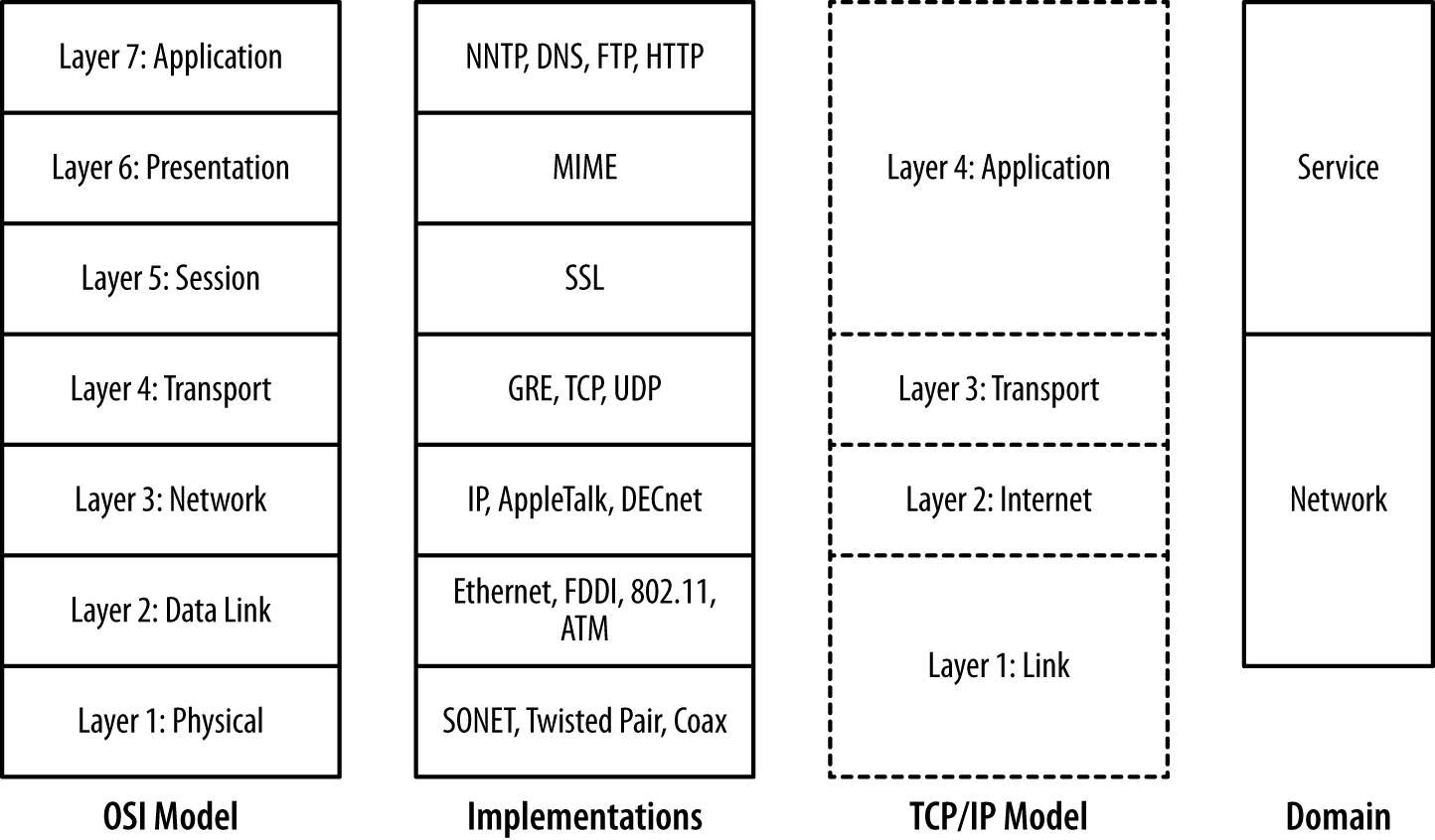
Figure 2-1. Layering models
The most common place where we encounter the impact of layering on network traffic is the maximum transmission unit (MTU). The MTU is an upper limit on the size of a data frame, and impacts the maximum size of a packet that can be sent over that medium. The MTU for Ethernet is 1,500 bytes, and this constraint means that IP packets will almost never exceed that size.
The layering model also provides us with a clear difference between the network and service-based sensor domains. As Figure 2-1 shows, network sensors are focused on layers 2 through 4 in the OSI model, while service sensors are focused on layers 5 and above.
Recall from Chapter 1 that a sensor’s vantage refers to the traffic that a particular sensor observes. In the case of computer networks, the vantage refers to the packets that a sensor observes either by virtue of transmitting the packets itself (via a switch or a router) or by eavesdropping (within a collision domain). Since correctly modeling vantage is necessary to efficiently instrument networks, we need to dive a bit into the mechanics of how networks operate.
Network Layers and Vantage
Network vantage is best described by considering how traffic travels at three different layers of the OSI model. These layers are across a shared bus or collision domain (layer 1), over network switches (layer 2), or using routing hardware (layer 3). Each layer provides different forms of vantage and mechanisms for implementing the same.
The most basic form of networking is across a collision domain. A collision domain is a shared resource used by one or more networking interfaces to transmit data. Examples of collision domains include a network hub or the channel used by a wireless router. A collision domain is called such because the individual elements can potentially send data at the same time, resulting in a collision; layer 2 protocols include mechanisms to compensate for or prevent collisions.
The net result is that layer 2 datagrams are broadcast across a common
source, as seen in Figure 2-2. Network interfaces on the same
collision domain all see the same datagrams; they elect to only
interpret datagrams that are addressed to them. Network capture tools
like tcpdump can be placed in promiscuous mode and
will then record all the datagrams observed within the collision
domain.
Figure 2-2 shows the vantage across collision domains. As seen in this figure, the initial frame (A to B) is broadcast across the hub, which operates as a shared bus. Every host connected to the hub can receive and react to the frames, but only B should do so. C, a compliant host, ignores and drops the frame. D, a host operating in promiscuous mode, records the frame. The vantage of a hub is consequently all the addresses connected to that hub.
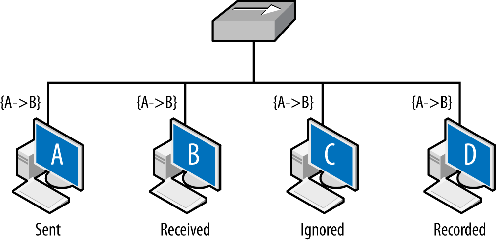
Figure 2-2. Vantage across collision domains
Shared collision domains are inefficient, especially with asynchronous protocols such as Ethernet. Consequently, layer 2 hardware such as Ethernet switches are commonly used to ensure that each host connected to the network has its own dedicated Ethernet port. This is shown in Figure 2-3.

Figure 2-3. Vantage across a switch
A capture tool operating in promiscuous mode will copy every frame that is received at the interface, but the layer 2 switch ensures that the only frames an interface receives are the ones explicitly addressed to it. Consequently, as seen in Figure 2-3, the A to B frame is received by B, while C and D receive nothing.
There is a hardware-based solution to this problem. Most switches implement some form of port mirroring. Port mirroring configurations copy the frames sent between different ports to common mirrored ports in addition to their original destination. Using mirroring, you can configure the switch to send a copy of every frame received by the switch to a common interface. Port mirroring can be an expensive operation, however, and most switches limit the amount of interfaces or VLANs monitored.
Switch vantage is a function of the port and the configuration of the switch. By default, the vantage of any individual port will be exclusively traffic originating from or going to the interface connected to the port. A mirrored port will have the vantage of the ports it is configured to mirror.
Layer 3, when routing becomes a concern, is when vantage becomes messy. Routing is a semiautonomous process that administrators can configure, but is designed to provide some degree of localized automation in order to provide reliability. In addition, routing has performance and reliability features, such as the TTL (described shortly), which can also impact monitoring.
Layer 3 vantage at its simplest operates like layer 2 vantage. Like switches, routers send traffic across specific ports. Routers can be configured with mirroring-like functionality, although the exact terminology differs based on the router manufacturer. The primary difference is that while layer 2 is concerned with individual Ethernet addresses, at layer 3 the interfaces are generally concerned with blocks of IP addresses because the router interfaces are usually connected via switches or hubs to dozens of hosts.
Layer 3 vantage becomes more complex when dealing with multihomed interfaces, such as the example shown in Figure 2-4. Up until this point, all vantages discussed in this book have been symmetric—if instrumenting a point enables you to see traffic from A to B, it also enables you to see traffic from B to A. A multihomed host like a router has multiple interfaces that traffic can enter or exit.
Figure 2-4 shows an example of multiple interfaces and their potential impact on vantage at layer 3. In this example, A and B are communicating with each other: A sends the packet {A→B} to B, B sends the packet {B→A} to A. C and D are monitoring at the routers: the top router is configured so that the shortest path from A to B is through it. The bottom router is configured so that shortest path from B to A is through it. The net effect of this configuration is that the vantages at C and D are asymmetric. C will see traffic from A to B, and D will see traffic from B to A, but neither of them will see both sides of the interaction. While this example is contrived, this kind of configuration can appear due to business relationships and network instabilities. It’s especially problematic when dealing with networks that have multiple interfaces to the internet.

Figure 2-4. Vantage when dealing with multiple interfaces
IP packets have a built-in expiration function: a field called the time-to-live (TTL) value. The TTL is decremented every time a packet crosses a router (not a layer 2 facility like a switch), until the TTL reaches 0 and the packet is dropped. In most cases, the TTL should not be a problem—most modern stacks set the TTL to at least 64, which is considerably longer than the number of hops required to cross the entire internet. However, the TTL is manually modifiable and there exist attacks that can use the TTL for evasion purposes. Table 2-1 lists default TTLs by operating system.1
| Operating system | TTL value |
|---|---|
Linux (2.4, 2.6) |
64 |
FreeBSD 2.1 |
64 |
macOS |
64 |
Windows XP |
128 |
Windows 7, Vista |
128 |
Windows 10 |
128 |
Solaris |
255 |
Figure 2-5 shows how the TTL operates. Assume that hosts C and D are operating on monitoring ports and the packet is going from A to B. Furthermore, the TTL of the packet is set to 2 initially. The first router receives the packet and passes it to the second router. The second router drops the packet; otherwise, it would decrement the TTL to 0. TTL does not directly impact vantage, but instead introduces an erratic type of blind spot—packets can be seen by one sensor, but not by another several routers later as the TTL decrements.

Figure 2-5. Hopping and router vantage
The net result of this is that the packet is observed by C, never received by B, and possibly (depending on the router configuration) observed at D.
Network Layers and Addressing
To access anything on a network, you need an address. Most hosts end up with multiple addresses at multiple layers, which are then moderated through different lookup protocols. For example, the host www.mysite.com may have the IP address 196.168.1.1 and the Ethernet address 0F:2A:32:AA:2B:14. These addresses are used to resolve the identity of a host at different abstraction layers of the network. For the analyst, the most common addresses encountered will be IPv4, IPv6, and MAC addresses.
In this section, I will discuss addressing in a LAN and instrumentation context. Additional information on addressing and lookup, primarily in the global context, is in Chapter 10.
MAC Addresses
A media access control (MAC) address is what the majority of layer 2 protocols, including Ethernet, FDDI, Token Ring, 802.11, Bluetooth, and ATM, use to identify a host. MAC addresses are sometimes called “hardware addresses,” as they are usually assigned as fixed values by hardware manufacturers.
MAC format and access
The most common MAC address format is MAC-48, a 48-bit integer. The canonical format for a MAC-48 is six zero-added two-digit hexadecimal octets separated by dashes (e.g., 01-23-45-67-89-AB), although colons and dropped padding are commonly seen (e.g., 1:23:45:67:89:AB).
MAC addresses are divided into two parts: the organizationally unique identifier (OUI), a 24-bit numeric ID assigned to the hardware manufacturer by the IEEE, followed by the NIC-specific element, assigned by the hardware manufacturer. The IEEE manages the registry of OUIs on its website, and there are a number of sites that will return a manufacturer ID if you pass them a MAC or full address.
IPv4-to-MAC lookup is managed using the Address Resolution Protocol (ARP).
IPv4 Format and Addresses
An IPv4 address is a 32-bit integer value assigned to every routable host, with exceptions made for reserved dynamic address spaces (see Chapter 10 for more information on these addresses). IPv4 addresses are most commonly represented in dotted quad format: four integers between 0 and 255 separated by periods (e.g., 128.1.11.3).
Historically, addresses were grouped into four classes: A, B, C, and D. A class A address (0.0.0.0–127.255.255.255) had the high order (leftmost) bit set to zero, the next 7 assigned to an entity, and the remaining 24 bits under the owner’s control. This gave the owner 224 addresses to work with. A class B address (128.0.0.0–191.255.255.255) assigned 16 bits to the owner, and class C (192.0.0.0–223.255.255.255) assigned 8 bits. This approach led rapidly to address exhaustion, and in 1993, Classless Inter-Domain Routing (CIDR) was developed to replace the naive class system.
Under the CIDR scheme, users are assigned a netblock via an address and a netmask. The netmask indicates which bits in the address the user can manipulate, and by convention, those bits are set to zero. For example, a user who owns the addresses 192.28.3.0–192.28.3.255 will be given the block 192.28.3.0/24. The suffix /24 here indicates that the high 24 bits are fixed, while the last 8 are open. /24s will contain 256 addresses, /27s 32, /16s 65,536, and so on.
A number of important IPv4 address blocks are reserved for special use. The IANA IPv4 Address Register contains a list of the most important /8s and their ownership. More important for administration and management purposes are the addresses listed in RFC 1918.2 The RFC 1918 local addresses define a set of IP addresses for local use, meaning that they can be used for internal networks (such as DHCP or NATed networks) that are not routed to the broader internet.3
IPv6 Format and Addresses
An IPv6 address is a 128-bit integer, solving the IPv4 address exhaustion problem by increasing the space by a factor of about 4 billion. By default, these addresses are described as a set of 16-bit hexadecimal groups separated by colons (e.g., 00AA:2134:0000:0000:A13F:2099:0ABE:FAAF). Given their length, IPv6 addresses use a number of conventions to shorten the representation. In particular:
-
Initial zeros are trimmed (e.g., AA:2134:0:0:A13F:2099:ABE:FAAF).
-
A sequence of zero-value groups can be replaced by empty colons (e.g., AA:2134:::A13F:2099:ABE:FAAF).
-
Multiple colons are reduced to a single pair (e.g., AA:2134::A13F:2099:ABE:FAAF).
As with IPv4, IPv6 blocks are grouped using CIDR notation. The IPv6 CIDR prefixes can be up to the full length of an IPv6 address (i.e., up to /128).
All of these relationships are dynamic, and multiple addresses at one layer can be associated with one address at another layer. As discussed earlier, a single DNS name can be associated with multiple IP addresses through the agency of the DNS service. Similarly, a single MAC address can support multiple IP addresses through the agency of the ARP protocol. This type of dynamism can be used constructively (like for tunneling) and destructively (like for spoofing).
Validity Challenges from Middlebox Network Data
Security analysts evaluating a network’s suitability for traffic analysis must consider not just whether they can see an address, but if they can trust it. Network engineers rely on a variety of tools and techniques to manage traffic, and the tools chosen can also affect vantage in a number of different ways.
We can categorize the general problems these tools introduce by how they impact analytics. In this section, I will discuss these effects and then relate them, in general and kind of loosely, to different common networking tools. Challenges to the validity of network data include threats to identity, causality, aggregation, consistency, and encryption. Table 2-2 shows how these are associated with the technologies we’ll discuss in the following subsections.
| Identity | Causality | Aggregation | Consistency | Encryption | |
|---|---|---|---|---|---|
NAT |
X |
X |
X |
||
DHCP |
X |
X |
|||
Load balancer |
X |
X |
|||
Proxy |
X |
X |
X |
X |
|
VPN |
X |
X |
X |
X |
These technologies will impact vantage, and consequently analysis, in a number of ways. Before we dig into the technologies themselves, let’s take a look at the different ways analytic results can be challenged by them:
- Identity
-
In some situations, the identity of individuals is not discernible because the information used to identify them has been remapped across boundaries—for example, a network address translator (NAT) changing address X to address Y. Identity problems are a significant challenge to internal validity, as it is difficult to determine whether or not the same individual is using the same address. Addressing identity problems generally requires collecting logs from the appliance implementing the identity mapping.
- Causality
-
Information after the middlebox boundary does not necessarily follow the sequence before the middlebox boundary. This is particularly a problem with caching or load balancing, where multiple redundant requests before the middlebox may be converted into a single request managed by the middlebox. This affects internal validity across the middlebox, as it is difficult to associate activity between the events before and after the boundary. The best solution in most cases is to attempt to collect data before the boundary.
- Aggregation
-
The same identity may be used for multiple individuals simultaneously. Aggregation problems are a particular problem for construct validity, as they affect volume and traffic measurements (for example, one user may account for most of the traffic).
- Consistency
-
The same identity can change over the duration of the investigation. For example, we may see address A do something malicious on Monday, but on Tuesday it’s innocent due to DHCP reallocation. This is a long-term problem for internal validity.
- Encryption
-
When traffic is contained within an encrypted envelope, deep packet inspection and other tools that rely on payload examination will not work.
DHCP
On DHCP (RFC 2131) networks—which are, these days, most networks—IP addresses are assigned dynamically from a pool of open addresses. Users lease an address for some interval, returning it to the pool after use.
DHCP networks shuffle IP addresses, breaking the relationship between an IP address and an individual user. The degree to which addresses are shuffled within a DHCP network is a function of a number of qualitative factors, which can result in anything from an effectively static network to one with short-term lifespans. For example, in an enterprise network with long leases and desktops, the same host may keep the same address for weeks. Conversely, in a coffee shop with heavily used WiFi, the same address may be used by a dozen machines in the course of a day.
While a DHCP network may operate as a de facto statically allocated network, there are situations where everything gets shuffled en masse. Power outages, in particular, can result in the entire network getting reshuffled.
When analyzing a network’s vantage, the analyst should identify DHCP networks, their size, and lease time. I find it useful to keep track of a rough characterization of the network—whether devices are mobile or desktops, whether the network is public or private, and what authentication or trust mechanisms are used to access the network. Admins should configure the DHCP server to log all leases, with the expectation that an analyst may need to query the logs to find out what asset was using what host at a particular time.
Sysadmins and security admins should also ask what assets are being allocated via DHCP. For critical assets or monitored users (high-value laptops, for example), it may be preferable to statically allocate an address to enable that asset’s traffic to be monitored via NetFlow or other network-level monitoring tools. Alternatively, critical mobile assets should be more heavily instrumented with host-based monitoring.
NAT
NATing (network address translation) converts an IP address behind a NAT into an external IP address/port combination outside the NAT. This results in a single IP address serving the interests of multiple addresses simultaneously. There are a number of different NATing techniques, which vary based on the number of addresses assigned to the NAT, among other things. In this case, we are going to focus on Port Address Translation (PAT), which is the most common form and the one that causes the most significant problems.
NATed systems both shuffle addresses (meaning that there is no realistic relationship between an IP address and a user) and multiplex them (meaning that the same address:port combination will rapidly serve multiple hosts). The latter badly affects any metrics or analyses depending on individual hosts, while the former confuses user identity. For this reason, the most effective solution for NATing is instrumentation behind the NAT.
Figure 2-6 shows this multiplexing in action. In this figure, you can see flow data as recorded from two vantage points: before and after translation. As the figure shows, traffic before the NAT has its own distinct IP addresses, while traffic after the NAT has been remapped to the NAT’s address with different port assignments.

Figure 2-6. NATing and proxies
Note that correlating NATing activity across both sides of the NAT requires the NAT itself to log that translation; this is discussed in more depth in Chapter 3.
Proxies
As with NATing, there are a number of different technologies (such as load balancing and reverse proxying) that fall under the proxy banner. Proxies operate at a higher layer than NATs—they are service-specific and, depending on the service in question, may incorporate load balancing and caching functions that will further challenge the validity of data collected across the proxy boundary.
Figure 2-6 shows how proxies remap traffic; as the figure shows, in a network with a proxy server, hosts using the proxy will always communicate with the proxy address first. This results in all communications with a particular service getting broken into two flows: client to proxy, proxy to server. This, in turn, exacerbates the differentiation problems introduced by NATing—if you are visiting common servers with common ports, they cannot be differentiated outside of the proxy, and you cannot relate them to traffic inside the proxy except through timing.
Without logs from the proxy, correlating traffic across proxy boundaries has extremely dubious validity. As with NATing, individual IP addresses and events are not differentiable. At the same time, internal instrumentation is not valuable because all the traffic goes to the same address. Finally, timing across proxies is always messy—web proxies, in particular, usually incorporate some form of caching to improve performance, and consequently the same page, fetched multiple times before the proxy, may be fetched only once after the proxy.
Load balancing
Load balancing techniques split traffic to a heavily used target between multiple servers and provide a common address to those servers. Load balancing can take place at multiple layers—techniques exist to remap DNS, IP, and MAC addresses as needed.
Load balancing primarily challenges identity and consistency, as the same address will, often very quickly, point to multiple different targets.
VPNs
In a virtual private network (VPN), some process wraps traffic in one protocol within the envelope of another protocol. Examples of these include classic VPN protocols such as Generic Routing Encapsulation (GRE), ad-hoc VPN tools such as Secure Shell (SSH), and transition protocols like Teredo or 6to4.
VPNs introduce two significant challenges. First, the encryption of the data in transit obviates deep packet inspection and any technique that requires examining or interpreting the payload. The other challenge is the identity problem—outside of the VPN, the observer sees a single, long-lived flow between client and VPN. At the VPN endpoint, the client will engage in multiple interactions with clients within the network, which are returned to the VPN access point and delivered to the client. The end result is a maze of IP address relationships across the VPN barrier.
Further Reading
-
R. Bejtlich, The Practice of Network Security Monitoring: Understanding Incident Detection and Response (San Francisco, CA: No Starch Press, 2003).
-
R. Bejtlich, The Tao of Network Security Monitoring: Beyond Intrusion Detection (Boston, MA: Addison-Wesley, 2004).
-
K. Fall and R. Stevens, TCP/IP Illustrated, Volume 1: The Protocols, 2nd ed. (Boston, MA: Addison-Wesley, 2011).
-
R. Perlman, Interconnections: Bridges, Routers, Switches, and Internetworking Protocols, 2nd ed. (Boston, MA: Addison-Wesley, 1999).
-
P. Goransson, C. Black, and T. Culver, Software Defined Networks: A Comprehensive Approach (Burlington, MA: Morgan Kaufmann, 2016).
1 A more comprehensive list of TTLs is maintained by Subin Siby at http://subinsb.com/default-device-ttl-values.
2 https://tools.ietf.org/html/rfc1918, updated by RFC 6761 at https://tools.ietf.org/html/rfc6761.
3 You will, of course, see them routed through the broader internet because nobody will follow BCP38 until the mutant cockroaches rule the Earth. You can learn about BCP38 at http://www.bcp38.info/. Go learn about BCP38, then go implement BCP38.