Chapter 2
The Error Component Model
The error component model is relevant when the slopes, i.e., the marginal effects of the covariates on the response, are the same for all the individuals, the intercepts being a priori different. Note that for some authors, the error component model is a byword for the “random‐effects model” as opposed to the “fixed‐effects model.” These two estimators will be analyzed in this chapter as two different ways to consider the individual component of the error terms for the same error component model (assuming no correlation and correlation with the regressors, respectively).
This is the landmark model of panel data econometrics, and this chapter presents the main results about it.
2.1 Notations and Hypotheses
2.1.1 Notations
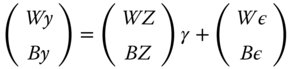
For the observation of individual ![]() at period
at period ![]() , we can write the model to be estimated, denoting by
, we can write the model to be estimated, denoting by ![]() the response,
the response, ![]() the vector of
the vector of ![]() covariates,
covariates, ![]() the error,
the error, ![]() the intercept, and
the intercept, and ![]() the vector of parameters associated to the covariates:
the vector of parameters associated to the covariates:
It'll be sometimes easier to store the intercept and the slopes in the same vector of coefficients. Denoting by ![]() this vector and
this vector and ![]() the associated vector of covariates, the model can then be written:
the associated vector of covariates, the model can then be written:
For the error component model, the error is the sum of two effects:
- the first,
 is the individual effect for individual
  ,
, - the second,
 is the residual effect, also called the idiosyncratic effect.
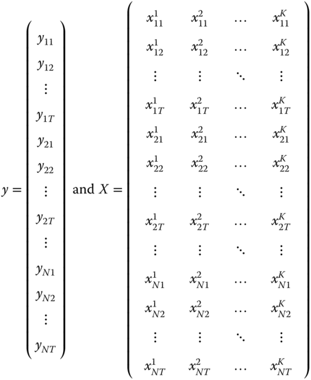
For the whole sample, we'll denote by ![]() the vector containing the response and
the vector containing the response and ![]() the matrix of covariates, storing the observations ordered by individual first and then by period. We'll suppose from now that the panel is balanced, which means that we have the same number of observations (
the matrix of covariates, storing the observations ordered by individual first and then by period. We'll suppose from now that the panel is balanced, which means that we have the same number of observations (![]() ) for all the individuals (
) for all the individuals (![]() ). In this case,
). In this case, ![]() is a vector of length
is a vector of length ![]() and
and ![]() a matrix of dimension
a matrix of dimension ![]() .
.
Denoting by ![]() a vector of ones of length
a vector of ones of length ![]() , we get:
, we get:
When we want to use the extended vector of coefficients, we denote ![]() , and the model to be estimated is:
, and the model to be estimated is:
2.1.2 Some Useful Transformations
Panel data econometricians usually break the total variation up into the sum of intra‐individual and inter‐individual variations. These two variations can easily be obtained by transforming the data using different transformation matrices, which can be written using Kronecker products.
The Kronecker product of 2 matrices, denoted ![]() , is the matrix obtained by multiplying each element of
, is the matrix obtained by multiplying each element of ![]() by
by ![]() .
.
![]() denotes the identity matrix of dimension
denotes the identity matrix of dimension ![]() ,
, ![]() is a vector of ones of length
is a vector of ones of length ![]() and
and ![]() is a matrix of 1 of dimension
is a matrix of 1 of dimension ![]() .
.
The inter‐individual (or between) transformation is obtained by using a transformation matrix denoted by ![]() , which is defined by:
, which is defined by:
For example, we have, for ![]() and
and ![]() :
:
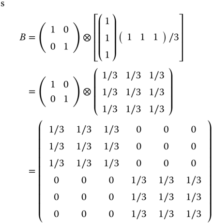
We then have:
To get the intra‐individual (or within) transformation, we'll use a transformation matrix ![]() defined as:
defined as:
These two matrices have very important properties:
- they are symmetric, so we then have
 and
and  ,
, - they are idempotent, which means that
 and
and  . For example, for the between transformation, if we apply it twice to
  , we obtain:
  . One computes the individual means of a vector, which already contains individual means; the vector is, therefore, unchanged; we then have
  , and the same reasoning applies to
  ,
, - they perform a decomposition of a vector, which means that
 , as
, as  and therefore
  ,
, - they are orthogonal:
 . Indeed, as the two matrices are symmetric and using the result that
  , we have:
  .
.  consist in taking the deviations from individual means of the individual means and is therefore equal to 0 irrespective of
  .
.
![]() and
and ![]() therefore perform an orthogonal decomposition of a vector
therefore perform an orthogonal decomposition of a vector ![]() ; this means that pre‐multiplying
; this means that pre‐multiplying ![]() by each of the two matrices, we obtain two vectors that sum to
by each of the two matrices, we obtain two vectors that sum to ![]() and for which the inner product is 0.
and for which the inner product is 0.
2.1.3 Hypotheses Concerning the Errors
![]() is the sum of a vector
is the sum of a vector ![]() of length
of length ![]() containing the idiosyncratic part of the error and of the individual effect
containing the idiosyncratic part of the error and of the individual effect ![]() , which is a vector of length
, which is a vector of length ![]() for which each element is repeated
for which each element is repeated ![]() times. This can be written in matrix form:
times. This can be written in matrix form:
The estimated model will be defined by estimated parameters ![]() and by a vector of residuals
and by a vector of residuals ![]() .
.
Subtracting 2.5 from 2.8 enables to write the residuals as a function of the errors:
To get a similar expression in terms of ![]() and
and ![]() , we use 2.4 and 2.7:
, we use 2.4 and 2.7:
The mean of this expression is, denoting ![]() :
:
In a linear model with an intercept, ![]() , which is the average of the residuals, is 0. Using the two previous equations, we get:
, which is the average of the residuals, is 0. Using the two previous equations, we get:
with ![]() a matrix that post‐multiplied by a vector returns a vector of the same length containing the overall mean.
a matrix that post‐multiplied by a vector returns a vector of the same length containing the overall mean. ![]() , post‐multiplied by a vector returns the vector in deviations from the overall mean.
, post‐multiplied by a vector returns the vector in deviations from the overall mean.
The expressions (2.9 and 2.10) will be used all along this chapter to analyze the properties of the estimators.
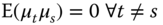
The following hypotheses are made concerning the errors:
- the expected values of the two components of the error are supposed to be 0; anyway, their means can't be identified if there is an intercept in the model,
- the individual effects
 are homoscedastic and mutually uncorrelated,
 - the idiosyncratic part of the error
 is also homoscedastic and uncorrelated,
 - the two components of the errors are uncorrelated.
In this case, the covariance matrix of the errors depends only on the variance of the two components of the errors, i.e., the two parameters ![]() and
and ![]() . Concerning the variance and covariances of the errors, we then have:
. Concerning the variance and covariances of the errors, we then have:
- for the variance of one error:
 ,
, - for the covariance of two errors of the same individual for two different periods:
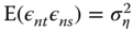 ,
, - for the covariance of two errors of two different individuals (belonging to the same period or not):
 .
.
For a given individual ![]() , the covariance matrix of the vector of errors for this individual
, the covariance matrix of the vector of errors for this individual ![]() is:
is:
For the whole sample, we have ![]() , and the covariance matrix is a square matrix of dimension
, and the covariance matrix is a square matrix of dimension ![]() that contains submatrices
that contains submatrices ![]() . For
. For ![]() , this submatrix is given by 2.11; for
, this submatrix is given by 2.11; for ![]() , this is a 0 matrix given the hypothesis of no correlation between the errors of two different individuals. The covariance matrix of the errors
, this is a 0 matrix given the hypothesis of no correlation between the errors of two different individuals. The covariance matrix of the errors ![]() is then a block‐diagonal matrix, the
is then a block‐diagonal matrix, the ![]() blocks being the matrix given by the equation 2.11. This matrix can then be expressed as a Kronecker product:
blocks being the matrix given by the equation 2.11. This matrix can then be expressed as a Kronecker product:
This matrix can also be usefully expressed in terms of the two transformation matrices within and between described in subsection 2.1.2. In fact, ![]() and
and ![]() . Introducing these two matrices in the expression of
. Introducing these two matrices in the expression of ![]() , we get:
, we get:
which finally implies, denoting ![]() :
:
Finally, all along this chapter, we'll suppose that both components of the errors are uncorrelated with the covariates: ![]() .
.
2.2 Ordinary Least Squares Estimators
The variability in a panel has two components:
- the between or inter‐individual variability, which is the variability of panel's variables measured in individual means, which is
 or, in matrix form,
  ,
, - the within or intra‐individual variability, which is the variability of panel's variables measured in deviation from individual means, which is
 or, in matrix form
  .
.
Three estimations by ordinary least squares can then be performed: the first one on raw data, the second one on the individual means of the data (between model), and the last one on the deviations from individual means (within model).
2.2.1 Ordinary Least Squares on the Raw Data: The Pooling Model
The model to be estimated is ![]() . Using the second formulation, the sum of squares residuals can be written:
. Using the second formulation, the sum of squares residuals can be written:
and the first‐order conditions for a minimum are (up to the ![]() multiplicative factor):
multiplicative factor):
The first column of ![]() is a vector of ones associated to
is a vector of ones associated to ![]() , which is the first element of
, which is the first element of ![]() . Therefore, dividing the first element of this vector by the number of observations leads to:
. Therefore, dividing the first element of this vector by the number of observations leads to:
This is the well‐known result that the mean of the sample, i.e., (![]() ) is on the regression line of the ordinary least squares estimator. The
) is on the regression line of the ordinary least squares estimator. The ![]() other first‐order conditions imply that
other first‐order conditions imply that ![]() , which can be rewritten, the average residual
, which can be rewritten, the average residual ![]() being equal to 0:
being equal to 0:
which means that the sample covariances between the residuals and the covariates are 0. Solving 2.13, we get the ordinary least squares estimator for the whole vector of coefficients:
Substituting ![]() by
by ![]() in 2.16,
in 2.16,
To get the estimator of the slopes, one splits ![]() in
in ![]() and
and ![]() in
in ![]() :
:
The formula for the inverse of a partitioned matrix is given by:

with ![]() . The upper left block may also be written:
. The upper left block may also be written: ![]()
We have here:
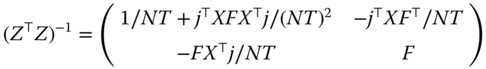
with ![]() .
. ![]() returns a vector of length
returns a vector of length ![]() for which all the elements are the vector mean
for which all the elements are the vector mean ![]() . One can easily check that this matrix is idempotent. We then have:
. One can easily check that this matrix is idempotent. We then have:
which is a formula similar to 2.16, but with variables pre‐multiplied by ![]() , this transformation removing the overall mean of every variable. For the intercept
, this transformation removing the overall mean of every variable. For the intercept ![]() , we find the same expression as 2.14. In order to analyze the characteristics of the OLS estimator, we substitute in 2.19
, we find the same expression as 2.14. In order to analyze the characteristics of the OLS estimator, we substitute in 2.19 ![]() by
by ![]() :
:
The estimator is then unbiased (![]() ) if
) if ![]() , i.e., if the theoretical covariances between the covariates and the errors are all 0. This result is directly linked with expression 2.13, which indicates that the OLS estimator is computed so that empirical covariances between the residuals and the covariates are all 0. The estimator is consistent if:
, i.e., if the theoretical covariances between the covariates and the errors are all 0. This result is directly linked with expression 2.13, which indicates that the OLS estimator is computed so that empirical covariances between the residuals and the covariates are all 0. The estimator is consistent if: ![]() . This expression is:
. This expression is:
The first term is the population covariance matrix of the covariates and the second one the population covariance vector of the covariates and the errors. The estimator is therefore consistent if the covariance matrix of the covariates exists, is not 0, and if the covariances between the covariates and the errors are all 0. The variance of the OLS estimator is given by:
Note that for the error component model, the covariance matrix of the errors ![]() doesn't reduce to a scalar times the identity matrix because of the correlation induced by the individual effects. Therefore, the variance of the OLS estimator doesn't reduce to
doesn't reduce to a scalar times the identity matrix because of the correlation induced by the individual effects. Therefore, the variance of the OLS estimator doesn't reduce to ![]() , and using this expression in tests will lead to biased inference.
, and using this expression in tests will lead to biased inference.
In conclusion, the OLS estimator, even if it is unbiased and consistent, has two limitations:
- the first one is that the usual estimator of the variance is not correct and should be replaced by a more complex expression,
- the second is that, in this context, OLS is not the best linear unbiased estimator, which means that there exist other linear unbiased estimators that are more efficient.
2.2.2 The between Estimator
The between estimator is the OLS estimator applied to the model pre‐multiplied by ![]() , i.e., the model in individual means.
, i.e., the model in individual means.
Note that the items of the model that don't exhibit intra‐individual variations are unaffected by this transformation. This is the case of the column of 1 associated to the intercept, of the matrix ![]() associated to the individual effects and also of some covariates with no intra‐individual as, for exemple, the gender in a sample of individuals. Note also that the
associated to the individual effects and also of some covariates with no intra‐individual as, for exemple, the gender in a sample of individuals. Note also that the ![]() observations of this model are in fact
observations of this model are in fact ![]() distinct observations of individual means repeated
distinct observations of individual means repeated ![]() times. Using as in the case of the OLS estimator, the formula of the inverse of a partitioned matrix, the between estimator is:
times. Using as in the case of the OLS estimator, the formula of the inverse of a partitioned matrix, the between estimator is:
![]() is a matrix that transforms a variable in its individual means in deviation from the overall mean. The variance of
is a matrix that transforms a variable in its individual means in deviation from the overall mean. The variance of ![]() is obtained by replacing
is obtained by replacing ![]() by
by ![]() :
:

The expression of ![]() given by 2.12 implies that
given by 2.12 implies that ![]() . Consequently, the expression of the variance of the between estimator is simply:
. Consequently, the expression of the variance of the between estimator is simply:
For the full vector of the coefficients (including the intercept ![]() ), the between estimator and its variance are:
), the between estimator and its variance are:
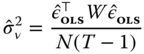
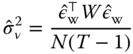
To estimate ![]() , we use the deviance of the between model:
, we use the deviance of the between model: ![]() . Using 2.23 and 2.9:
. Using 2.23 and 2.9:

The ![]() matrix is idempotent, and its trace is, using the property that the trace is invariant under cyclical permutations:
matrix is idempotent, and its trace is, using the property that the trace is invariant under cyclical permutations: ![]() . We then have
. We then have ![]() and
and ![]() . The unbiased estimator of
. The unbiased estimator of ![]() is then
is then ![]() . The one returned by an OLS program is:
. The one returned by an OLS program is: ![]() and the covariance matrix of the coefficients should then be multiplied by
and the covariance matrix of the coefficients should then be multiplied by ![]() .
.
2.2.3 The within Estimator
The within estimator is obtained by applying the OLS estimator to the model pre‐multiplied by the ![]() matrix.
matrix.
The within transformation removes the vector of 1 associated to the intercept and the matrix associated to the vector of individual effects. It also removes covariates that don't exhibit intra‐individual variation. Applying OLS to the transformed model leads to the within estimator:
The variance of ![]() is:
is:
![]() . The within transformation therefore induces a correlation among the errors of the model. The variance of the within estimator reduces to:
. The within transformation therefore induces a correlation among the errors of the model. The variance of the within estimator reduces to:
we then have, in spite of this correlation, the standard expression of the variance. In order to estimate ![]() , one uses the deviance of the within estimator:
, one uses the deviance of the within estimator: ![]() . Using 2.25 and 2.10:
. Using 2.25 and 2.10:
The matrix ![]() is idempotent and its trace is
is idempotent and its trace is ![]() . We then have
. We then have ![]() . The unbiased estimator of
. The unbiased estimator of ![]() is then
is then ![]() , and the one returned by an OLS program is:
, and the one returned by an OLS program is: ![]() . The covariance matrix of the coefficients should then be multiplied by:
. The covariance matrix of the coefficients should then be multiplied by: ![]() .
.
The within model is also called the “fixed‐effects model” or the least‐squares dummy variable model, because it can be obtained as a linear model in which the individual effects are estimated and then taken as fixed parameters. This model can be written:
where ![]() is now a vector of parameters to be estimated. There are therefore
is now a vector of parameters to be estimated. There are therefore ![]() parameters to estimate in this model.1 The estimation of this model is computationally feasible if
parameters to estimate in this model.1 The estimation of this model is computationally feasible if ![]() is not too large. In a micro panel of large size, the estimation becomes problematic.
is not too large. In a micro panel of large size, the estimation becomes problematic.
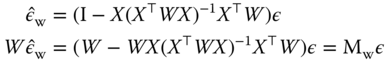
The equivalence between both models may be established using the Frisch‐Waugh theorem or using the formula of the inverse of a partitioned matrix. The Frisch‐Waugh theorem states that it is equivalent to regress ![]() on a set of covariates
on a set of covariates ![]() or to regress the residuals of
or to regress the residuals of ![]() from a regression on
from a regression on ![]() on the residuals of
on the residuals of ![]() on a regression on
on a regression on ![]() . The application of the Frisch‐Waugh theorem in this context consists in regressing each variable with respect to
. The application of the Frisch‐Waugh theorem in this context consists in regressing each variable with respect to ![]() and getting the residuals. Here, for each variable, the residual is
and getting the residuals. Here, for each variable, the residual is ![]() . The first‐order condition of the sum of squared residuals minimization is
. The first‐order condition of the sum of squared residuals minimization is ![]() .
. ![]() being a matrix which selects the individuals, we finally get for every individual, denoting
being a matrix which selects the individuals, we finally get for every individual, denoting ![]() :
:

Consequently, we have ![]() and the residuals are the deviations of the variable from its individual means. Therefore, the Frisch‐Waugh theorem implies that the fixed effect model can be estimated by applying the OLS estimator to the model transformed in deviations from the individual means, i.e., by regressing
and the residuals are the deviations of the variable from its individual means. Therefore, the Frisch‐Waugh theorem implies that the fixed effect model can be estimated by applying the OLS estimator to the model transformed in deviations from the individual means, i.e., by regressing ![]() on
on ![]() .
.
With the within coefficients in hand, specific intercepts for every individual in the sample ![]() can then be computed:
can then be computed:
where ![]() is the vector of individual means of
is the vector of individual means of ![]() .
.
If one wants to define individual effects with 0 mean in the sample, a general intercept can be computed: ![]() ,
, ![]() being the overall mean of
being the overall mean of ![]() . We then have for every individual in the sample
. We then have for every individual in the sample ![]()
2.3 The Generalized Least Squares Estimator
The within estimator is a regression on data that have been transformed so that the individual effects vanish (they are, so to say, “transformed out”), while the least squares dummy variables considers the individual effects as parameters to be estimated (they are “estimated out”); both give identical estimates of the slopes. On the contrary, the GLS estimator considers the individual effects as random draws from a specific distribution and seeks to estimate the parameters of this distribution in order to obtain efficient estimators of the slopes.
2.3.1 Presentation of the GLS Estimator
When the errors are not correlated with the covariates but are characterized by a non‐scalar covariance matrix ![]() , the efficient estimator is the generalized least squares estimator:
, the efficient estimator is the generalized least squares estimator:
In order to compute the variance of ![]() , we substitute as previously
, we substitute as previously ![]() by
by ![]() . We then have:
. We then have:
Using a reasoning similar to 2.20, we obtain the variance of the estimator:

The hypothesis we have made concerning the errors implies that the covariance matrix of the errors is given by 2.12: ![]() , which is a linear combination of two idempotent and orthogonal matrices.
, which is a linear combination of two idempotent and orthogonal matrices. ![]() depends only on two parameters: the variances of the two components of the error terms (
depends only on two parameters: the variances of the two components of the error terms (![]() and
and ![]() ). We have shown, in subsection 2.1.2, that these two matrices are idempotent (
). We have shown, in subsection 2.1.2, that these two matrices are idempotent (![]() and
and ![]() ) and orthogonal (
) and orthogonal (![]() ). The expression of powers of
). The expression of powers of ![]() is then particularly simple:
is then particularly simple:
which can be easily checked, for example for ![]() . This result can also be extended to negative integers and to rationals; we then have, for
. This result can also be extended to negative integers and to rationals; we then have, for ![]() :
:
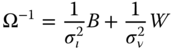
and the GLS estimator of the random error model and its variance are then:


For the vector of slopes, we obtain:

This estimator is called the random effects model, as opposed to the fixed effects model. This results from the fact that, as observed, in this case, the individual effects are considered as random deviates, the parameters of whose distribution we seek to estimate.
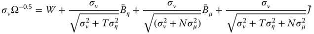
The dimension of the matrix ![]() is given by the size of the sample. If the sample is large, it is therefore not practical to compute the estimator according to the matrix formula 2.27. A more efficient way is to apply OLS on suitably pre‐transformed data. To this end, one has to compute the
is given by the size of the sample. If the sample is large, it is therefore not practical to compute the estimator according to the matrix formula 2.27. A more efficient way is to apply OLS on suitably pre‐transformed data. To this end, one has to compute the ![]() matrix such that:
matrix such that: ![]() and then use this matrix to transform all the variables of the model. Denoting
and then use this matrix to transform all the variables of the model. Denoting ![]() and
and ![]() the transformed variables, the estimation by OLS on transformed variables gives:
the transformed variables, the estimation by OLS on transformed variables gives:
which is the GLS given by 2.30. The expression of the matrix ![]() is obtained using equation 2.29 for
is obtained using equation 2.29 for ![]() :
:
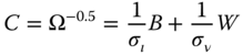
This transformation consists in a linear combination of the between and within transformations with weights depending on the variances of the two error components. In fact, pre‐multiplying the variables by ![]() (which is equivalent to premultiplication by
(which is equivalent to premultiplication by ![]() and simplifies notation), the weights become respectively
and simplifies notation), the weights become respectively ![]() and 1. The transformed variable is therefore:
and 1. The transformed variable is therefore:
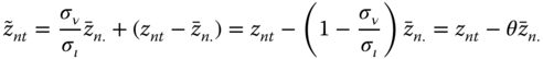
with, denoting ![]() :
:

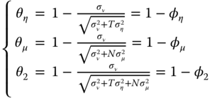
As will be explained in detail below, the importance of the individual effects in the composite errors, measured by their share of the total variance, determines how close the estimator will be to either the within or the pooled OLS, which are obtained as special cases, respectively, when the variance of the individual effects ![]() dominates (
dominates (![]() ) or vanishes (
) or vanishes (![]() ).
).
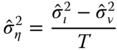
2.3.2 Estimation of the Variances of the Components of the Error
In order to make operational the estimator, residuals from consistent estimators are used to estimate the unknown parameters ![]() and
and ![]() (and hence
(and hence ![]() ). The estimator obtained is then called the feasible generalized least squares estimator.
). The estimator obtained is then called the feasible generalized least squares estimator.
Consider the errors of the model ![]() , their individual mean
, their individual mean ![]() and their deviations from these individual means
and their deviations from these individual means ![]() . By hypothesis, we have:
. By hypothesis, we have: ![]() . For the individual means, we get:
. For the individual means, we get:

The variance of the deviation from the individual means is easily obtained by isolating terms in ![]() :
:
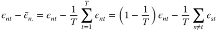
the sum then contains ![]() terms. The variance is:
terms. The variance is:
which finally leads to:
If ![]() were known, natural estimators of these two variances
were known, natural estimators of these two variances ![]() et
et ![]() would be:
would be:

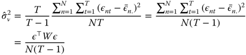
i.e., estimators based on the norm of the errors transformed using the between and within matrices. Of course, the errors are unknown, but consistent estimation of the variances may be obtained by substituting the errors by residuals obtained from a consistent estimation of the model. Among the numerous estimators available, the one proposed by Wallace and Hussain (1969) is particularly simple as it consists on using the OLS residuals to write the sample counterpart of equations 2.34 and 2.35

The estimated variance of the individual effects can then be obtained:
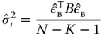
The estimator of Amemiya (1971) is based on the estimation of the within model. We first compute the overall intercept
and then compute the residuals ![]() :
:
These residuals are then used to compute the two quadratic form.

Note that the later is just the deviance of the within estimation divided by ![]() . Note also that the variance of the individual effect is overestimated if the model contains some time‐invariant variables which disappear with the within transformation.
. Note also that the variance of the individual effect is overestimated if the model contains some time‐invariant variables which disappear with the within transformation.
In this case, Hausman and Taylor (1981) proposed the following adjustment: ![]() are regressed on all the time‐invariant variables in the model and the residuals of this regression
are regressed on all the time‐invariant variables in the model and the residuals of this regression ![]() are substituted with
are substituted with ![]() in the computation of the quadratic forms. This will reduce the estimate of
in the computation of the quadratic forms. This will reduce the estimate of ![]() and leave unchanged the estimate of
and leave unchanged the estimate of ![]() , so that the estimate of
, so that the estimate of ![]() will also decrease.
will also decrease.
For the Swamy and Arora (1972) estimator, the within and the between models are estimated. The residuals of the between model are used for the first quadratic form and those of the within model for the second one.

Note that Swamy and Arora (1972) use the degrees of freedom of both regressions for the estimation of the variances, i.e., ![]() is deduced from the number of observations. Note also that
is deduced from the number of observations. Note also that ![]() and
and ![]() are the residuals of the between and within regressions computed on the transformed data, so that the numerators of the two quadratic forms are the deviances of the two regressions.
are the residuals of the between and within regressions computed on the transformed data, so that the numerators of the two quadratic forms are the deviances of the two regressions.
For all these estimators, ![]() is not directly estimated but obtained by subtracting
is not directly estimated but obtained by subtracting ![]() from
from ![]() . In small samples, it can therefore be negative, and in this case it is set to 0.
. In small samples, it can therefore be negative, and in this case it is set to 0.
On the contrary, for the Nerlove (1971) estimator, ![]() is estimated by computing the empirical variance of the fixed effects of the within model, as the estimate of
is estimated by computing the empirical variance of the fixed effects of the within model, as the estimate of ![]() is obtained by dividing the quadratic form of the within residuals by the number of observations.
is obtained by dividing the quadratic form of the within residuals by the number of observations.

2.4 Comparison of the Estimators
We have four different estimators of the same model : the between and the within estimators use only one source of the variance of the sample, while the OLS and the GLS estimators use both.
Note first that, if the hypothesis that the errors and the covariates are uncorrelated is true, all these models are unbiased and consistent, which means that they should give similar results, at least in large samples.
We'll first analyze the relations between these estimators; we'll then compare their variances; and finally we'll analyze in which circumstances we should use fixed or random effects.
2.4.1 Relations between the Estimators
We can expect the OLS and GLS estimators to give intermediate results between the within and the between estimators as they use both sources of variance. From equation 2.32, the GLS estimator can be written :
Using 2.21 and 2.25, ![]() can then be expressed as a weighted average of the within and the between estimators.
can then be expressed as a weighted average of the within and the between estimators.
A similar result applies to the OLS estimator which is the GLS estimator for ![]() .
.
For the OLS estimator, the weights are very intuitive because they are just the shares of the intra‐ and the inter‐individual variances of the covariates. For the GLS estimator, the weights depend not only on the shares of the variance of the covariates but also on the variance of the errors, which determines the ![]() parameter. The GLS estimator will always give less weight to the between variation, as
parameter. The GLS estimator will always give less weight to the between variation, as ![]() is lower than 1. It leads to two special cases :
is lower than 1. It leads to two special cases :
 ; this means that
  is “small” compared to
  . In this case, the GLS estimator converges to the within estimator,
 ; this means that
  is “large” compared to
  . In this case, the GLS estimator converges to the OLS estimator.
The relation between the estimators can also be illustrated by the fact that the OLS and the GLS can be obtained by stacking the within and between transformations of the model:2
The matrix of covariance of the errors of this stacked model is :

Applying OLS to 2.36, we get;
which is the OLS estimator,
while applying GLS to 2.36 yields the GLS estimator of equation 2.30.
2.4.2 Comparison of the Variances
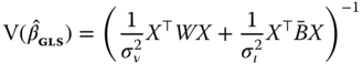
From equation 2.33, the variance of the GLS estimator can be written :
The variance of the within estimator being : ![]() ,
, ![]() is a positive definite matrix, and the GLS estimator is therefore more efficient than the within estimator. Similarly, equation 2.22 shows that the variance of the between may be written
is a positive definite matrix, and the GLS estimator is therefore more efficient than the within estimator. Similarly, equation 2.22 shows that the variance of the between may be written ![]() and therefore
and therefore ![]() is also a positive definite matrix.
is also a positive definite matrix.
2.4.3 Fixed vs Random Effects
The individual effects are not fixed or random by nature. Within the same framework (the individual effects model), they are treated as either a vector of constant parameters or the realization of random deviates for the purpose of estimation, depending on their probabilistic structure and, in particular, on their correlation with the explanatory variables.
In a micro‐panel, the random effects approach is appealing, as we work on a sample with numerous individuals who are randomly drawn from a very large population. There is no interest in estimating the individual effects, and the random effect approach is more appropriate, given the way the sample was obtained.
On the contrary, in a macro‐panel, the sample is fixed or quasi‐fixed and almost exhaustive (think of the countries of the world or the large enterprises of a country). In this case, the estimation of the individual effects may be an interesting result, and the fixed effects approach seems relevant.
Anyway, the main argument that leads to choose one of the two approaches is the possibility of correlation between some covariates and the individual effects. If we maintain the hypothesis that the idiosyncratic error is uncorrelated with the covariates (![]() ), two situations can occur :
), two situations can occur :
 : the individual effects are not correlated; in this case, both models are consistent, but the random effects estimator is more efficient that the fixed effects model,
 : the individual effects are correlated; in this case, only the fixed effects method gives consistent estimates as, with the within transformation, the individual effects vanish.
2.4.4 Some Simple Linear Model Examples
Even if they are of limited practical interest, given that relevant econometric models usually contain several covariates, simple linear models have a great pedagogical value, as they enable the graphical representation of the sample and estimators using regression lines. They are for this reason very useful to illustrate the relationship between the estimators. We'll use successively four data sets.
2.5 The Two‐ways Error Components Model
The two‐ways error component is obtained by adding a time‐invariant effect ![]() to the model.
to the model.
2.5.1 Error Components in the Two‐ways Model
We make for the time effects the same hypotheses that we made for the individual effects:
 has a zero mean and is homoscedastic, its variance is denoted by
  ,
,- the time effects are mutually uncorrelated,
 ,
, - the time effects are uncorrelated with the individual effects and the idiosyncratic terms.
With these hypotheses, the covariance matrix of the errors becomes:
As for the individual error component model, we write this covariance matrix as a linear combination of idempotent and mutually orthogonal matrices. To this aim, we write:
![]() computes, as before, the individual means
computes, as before, the individual means ![]() ,
, ![]() the time means
the time means ![]() and
and ![]() the overall mean
the overall mean ![]() . Finally, the within matrix now produces deviations from the individual and the time means:
. Finally, the within matrix now produces deviations from the individual and the time means: ![]() :
:
With these notations, we get:
It can be easily checked that these matrices are idempotent. On the contrary, they are not all orthogonal, as ![]() . The product of these two matrices allows to compute the time means of the individual means, which results in the overall mean. For this reason, we use
. The product of these two matrices allows to compute the time means of the individual means, which results in the overall mean. For this reason, we use ![]() and
and ![]() , which return respectively the individual and the time means in deviations from the overall mean. We finally obtain:
, which return respectively the individual and the time means in deviations from the overall mean. We finally obtain:
2.5.2 Fixed and Random Effects Models
As for the individual effects model, the two‐ways fixed effects model can be obtained in two different ways:
- by estimating by OLS the model that includes individual and time dummies,
- by estimating by OLS the model where all the variables have been transformed in deviations from the individual and the time means:
 .
.
For the GLS model the variables are pre‐multiplied by ![]() or more simply by:
or more simply by:
Collecting terms, we obtain the following expression for the transformed data:
with: