
Chapter 3
Advanced Error Components Models
3.1 Unbalanced Panels
For unbalanced panels, the number of observations for each individual is now individual specific and denoted by ![]() . We'll denote by
. We'll denote by ![]() the total number of observations. Compared to the balanced panel case, three complications appear:
the total number of observations. Compared to the balanced panel case, three complications appear:
- firstly, the covariance matrix of the errors cannot be written any more as a linear combination of idempotent and mutually orthogonal matrices (for the one‐way error component model, the within and the between matrices), the weights being the variances of the errors (
 and
and  ). Denoting by
  and
and  two matrices of individual and time dummies, matrices of the type
  , returning either the sum of the values for an individual or for a time series, will explicitly appear, and these matrices are not idempotent;
 - secondly, for the individual effects model, the within transformation still consists of removing the individual mean from the variable. On the contrary, for the two‐ways effects, the within transformation is not obtained by performing a difference with the individual and time means, as in the balanced panel case, but requires more tedious matrix algebra;
- finally, to estimate the components of the variance, we will still compute quadratic forms of the residuals of some consistent preliminary estimations, but there is no obvious choice of denominators, as there was in the balanced case.
3.1.1 Individual Effects Model
The model to be estimated can be written:
The fixed effects model may be estimated by regressing ![]() on
on ![]() and
and ![]() . Like in the balanced panel case, the Frisch‐Waugh theorem enables to avoid the estimation of the fixed effects. The estimation of
. Like in the balanced panel case, the Frisch‐Waugh theorem enables to avoid the estimation of the fixed effects. The estimation of ![]() may be obtained by regressing in a first stage
may be obtained by regressing in a first stage ![]() and
and ![]() on
on ![]() , computing the residuals and then regressing in the second stage the residuals of
, computing the residuals and then regressing in the second stage the residuals of ![]() on those of
on those of ![]() . As in the balanced panel case, these residuals are just the individual within transformation, i.e.,
. As in the balanced panel case, these residuals are just the individual within transformation, i.e., ![]() or
or ![]() in matrix form, and the fixed effects model is simply obtained by regressing
in matrix form, and the fixed effects model is simply obtained by regressing ![]() on
on ![]() .
.
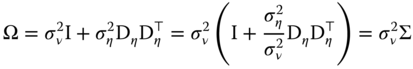
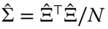
For the GLS model, the covariance matrix of the errors is:
The GLS estimator writes:
![]() is a block‐diagonal matrix that contains
is a block‐diagonal matrix that contains ![]() square matrices of ones of dimension
square matrices of ones of dimension ![]() . For balanced panels,
. For balanced panels, ![]() and
and ![]() .
. ![]() returns the sum of the values of
returns the sum of the values of ![]() for each individual.
for each individual. ![]() is also a block‐diagonal matrix, with blocks
is also a block‐diagonal matrix, with blocks ![]() of the form:
of the form:
with ![]() .
.
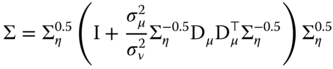
The inverse of a block‐diagonal matrix being equal to a block‐diagonal matrix for which the blocks are the inverses of those of the initial matrix, it is sufficient to calculate the inverse of ![]() . As it is a linear combination of two idempotent and orthogonal matrices, the general formula for any power of
. As it is a linear combination of two idempotent and orthogonal matrices, the general formula for any power of ![]() is:
is:

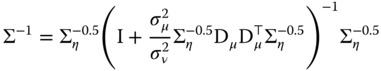
In particular, the inverse is:

which can also be written as ![]() , with:
, with:

The GLS estimator may then be obtained by applying OLS on variables that have been transformed by pre‐multiplying them by ![]() or, equivalently, by
or, equivalently, by ![]() (which will simplify notation):
(which will simplify notation):
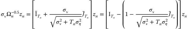
As in the balanced case, the transformed data can be expressed as quasi‐differences, ![]() , with:
, with:
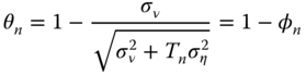
the only difference being that now, the proportion of the individual mean that is removed is not a constant, as it depends on the number of observations for each individual.
3.1.2 Two‐ways Error Component Model
For the two‐ways error component model, we have:
or, in matrix form:
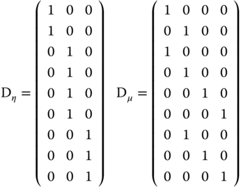
where ![]() and
and ![]() are matrices of respectively individual and time dummies. Pre‐multiplying a vector by
are matrices of respectively individual and time dummies. Pre‐multiplying a vector by ![]() and
and ![]() returns, respectively, the individual and time sum of the variable.
returns, respectively, the individual and time sum of the variable.
![]() and
and ![]() are two diagonal matrices that contain the number of observations for each individual and time‐series. Pre‐multiplying a vector by
are two diagonal matrices that contain the number of observations for each individual and time‐series. Pre‐multiplying a vector by ![]() or by
or by ![]() returns, respectively, the individual and the time series means. Finally,
returns, respectively, the individual and the time series means. Finally, ![]() is a
is a ![]() matrix of ones and zeros, which indicates whether an observation for a specific individual and time period is present or not.
matrix of ones and zeros, which indicates whether an observation for a specific individual and time period is present or not.
To help visualizing these matrices, we consider a panel with 3 individuals and 4 periods; the panel is unbalanced, as the first individual is not observed in the third and fourth periods, and the third one is not observed in the first period.


3.1.2.1 Fixed Effects Model
The fixed effects model can be estimated regressing ![]() on
on ![]() and the two matrices associated with the effects vectors
and the two matrices associated with the effects vectors ![]() and
and ![]() .
.
The application of the Frisch‐Waugh theorem implies that the estimation can be performed by regressing in a first stage ![]() ,
, ![]() , and
, and ![]() on
on ![]() and then, in a second stage, by regressing the residuals of
and then, in a second stage, by regressing the residuals of ![]() on those of
on those of ![]() and
and ![]() , which means regressing
, which means regressing ![]() on
on ![]() and
and ![]() .
.
Applying the same theorem again, one can regress in ![]() and
and ![]() on
on ![]() in the first stage, and the residuals of
in the first stage, and the residuals of ![]() on those of
on those of ![]() in the second stage.
in the second stage.
Residuals of a regression on ![]() are obtained by pre‐multiplying the variables by the matrix:
are obtained by pre‐multiplying the variables by the matrix:
where, for any matrix ![]() ,
, ![]() is the generalized inverse of
is the generalized inverse of ![]() . Finally, the two‐ways error component fixed effects model may be obtained by applying to
. Finally, the two‐ways error component fixed effects model may be obtained by applying to ![]() and every column of
and every column of ![]() the following transformation:
the following transformation:
The double‐within transformation consists then, for unbalanced panels, in multiplying any data vector by the following matrix:
Therefore, the two‐ways fixed effects model is still easy to compute even if the panel is unbalanced: all that is required is OLS estimation and the computation of deviations from the individual means. One proceeds as follows:
- first, the individual within transformation is applied to
 ,
,  and
and  ,
, - next,
 and
and  are regressed on
  ,
, - finally, from these regressions, the residuals of
 and
and  are obtained; then the residuals of the latter are regressed on those of the former.
The within transformation is performed on ![]() variables, and then
variables, and then ![]() preliminary linear estimations are performed on
preliminary linear estimations are performed on ![]() covariates before the final estimation for which there are
covariates before the final estimation for which there are ![]() covariates.
covariates.
Note that no specific matrix computation is required and that, in particular, the matrix of individual dummies, which is often very large (![]() ), need not to be stored during the estimation.
), need not to be stored during the estimation.
3.1.2.2 Random Effects Model
The variance matrix of the errors is:
with:
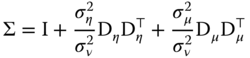
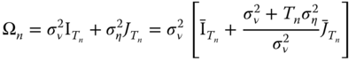
Denote ![]() the covariance matrix of the errors of the individual one‐way error components model. We then have:
the covariance matrix of the errors of the individual one‐way error components model. We then have:
![]() is block‐diagonal, with blocks:
is block‐diagonal, with blocks: ![]() .
. ![]() and
and ![]() being idempotent and orthogonal, the matrix
being idempotent and orthogonal, the matrix ![]() (defined so that
(defined so that ![]() ) is also a block‐diagonal matrix with blocks:
) is also a block‐diagonal matrix with blocks:  . We then have:
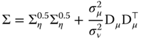
for which the inverse is:
We then apply the following result: ![]() to the matrix in brackets:
to the matrix in brackets:

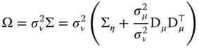
Finally, we have:

and the GLS estimator is:
Let ![]() and
and ![]() the matrix of the covariates and of the time dummies measured in quasi‐difference from the individual means. We then have:
the matrix of the covariates and of the time dummies measured in quasi‐difference from the individual means. We then have:
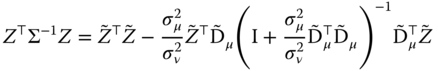
and a similar expression for ![]() . With the two matrices
. With the two matrices ![]() and
and ![]() in hand, the computation of the estimator requires:
in hand, the computation of the estimator requires:
- computing the cross products of the two matrices
 ,
,  and
and  ,
, - computing the inverse of a matrix of dimension
 .
.
These are reasonable computational tasks: note especially that the matrix of individual effects needn't be stored and that the dimension of the matrix that has to be inverted is ![]() and not
and not ![]() or
or ![]() and that, at least for micro‐panels,
and that, at least for micro‐panels, ![]() is relatively small. Note also that computation of the GLS estimator requires explicit matrix operations and it can no longer be obtained as a series of linear regressions on transformed data.
is relatively small. Note also that computation of the GLS estimator requires explicit matrix operations and it can no longer be obtained as a series of linear regressions on transformed data.
3.1.3 Estimation of the Components of the Error Variance
Remember that, in the balanced panel case, we used the result that natural estimators of ![]() and
and ![]() were:
were:

Feasible estimates were obtained by replacing ![]() by the residuals
by the residuals ![]() from a consistent estimation. For the balanced case,
from a consistent estimation. For the balanced case, ![]() and
and ![]() were natural denominators. This is no longer the case when the panel is unbalanced, as
were natural denominators. This is no longer the case when the panel is unbalanced, as ![]() is not the same for all individuals (and
is not the same for all individuals (and ![]() is not the same for all time periods).
is not the same for all time periods).
The strategy used here consists in computing the expected values of the quadratic forms in order to obtain unbiased estimators of the variance components:
- first, for a given estimator, define the matrix
 that transforms the errors into the residuals of the
  estimator:
  ,
, - compute the two quadratic forms of the within and between transformation of the residuals:
 and
and 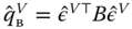 (
( and
and 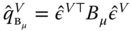 for the two‐ways error component model).
 - compute the expected values of these quadratic forms, which are functions of
 ,
,  (and
(and  for the two‐ways model),
 - equate the quadratic forms to their expected values and solve the system of two (or three equations for the two‐ways error component model) for
 ,
,  (and
(and  in the latter case).
Different estimators are obtained using different preliminary models to obtain the residuals. Among the numerous possible choices, as previously seen on chapter 2:
- Wallace and Hussain (1969) use the residuals of the pooling estimator for the two quadratic forms,
- Amemiya (1971) use the residuals of the OLS estimator for the two quadratic forms,
- Swamy and Arora (1972) use the residuals of the OLS estimator for the first quadratic form and those of the OLS estimator for the second one.
The model and its estimation are:
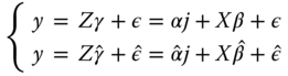
The intercept can be removed by pre‐multiplying every element of the model by: ![]() , which subtracts from every variable its overall mean and therefore removes the intercept, as
, which subtracts from every variable its overall mean and therefore removes the intercept, as ![]() .
.
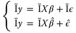
Subtracting the expression of the model and of its estimation, we get:
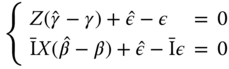
The three estimators we use (OLS, within, and between) can be seen as GLS estimators of this model, with ![]() being equal, respectively, to
being equal, respectively, to ![]() ,
, ![]() , and
, and ![]() :
:

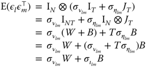
Using the two previous expressions, we get ![]() with:
with:
![]() is the matrix that transforms the error vector into the residuals vector. Note that it is not a symmetric matrix, at least unless
is the matrix that transforms the error vector into the residuals vector. Note that it is not a symmetric matrix, at least unless ![]() (which corresponds to the pooling model). The quadratic form of the residuals with a matrix
(which corresponds to the pooling model). The quadratic form of the residuals with a matrix ![]() is:
is:
![]() being a scalar, it is also equal to its trace:
being a scalar, it is also equal to its trace:
Using the cyclic property of the trace operator, we get:
from which, taking expectations, we obtain:
with ![]() .
.
Finally, we get:
Replacing ![]() by its expression and denoting
by its expression and denoting ![]() , we get:
, we get:

or, denoting ![]() :
:

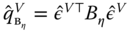
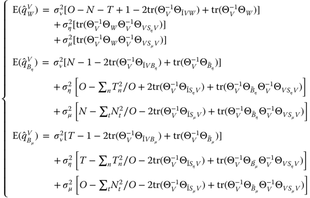
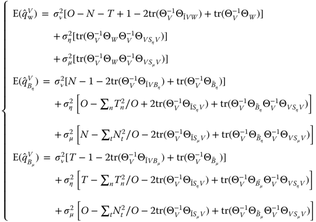
The most common estimators are obtained by considering the quadratic forms with the within, between‐individual, and between‐time matrices. We then get the following system of equations:
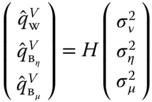
with

Using the following results: ![]() ,
, ![]() ,
, ![]() ,
, ![]() ,
, ![]() ,
, ![]() ,
, ![]() ,
, ![]() ,
, ![]() ,
, ![]() and
and ![]() ,
, ![]() and
and ![]() ,
, ![]() ,
, ![]() ,
, ![]() ,
, ![]() ,
, ![]() ,
, ![]() , we get:
, we get:
or:

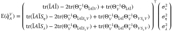
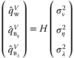
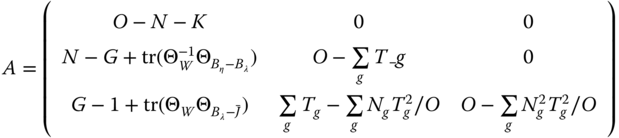
The estimator is obtained by equating the quadratic form and its expected value:
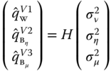
The ![]() matrices corresponding to the three most common estimators are presented in Figure 3.1.
matrices corresponding to the three most common estimators are presented in Figure 3.1.
Amemiya (1971):
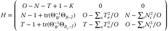
Wallace and Hussain (1969):
Swamy and Arora (1972):

Figure 3.1Estimators of the variance components for unbalanced panels.
3.2 Seemingly Unrelated Regression
3.2.1 Introduction
Very often in economics, the phenomenon under investigation is not well described by a single equation but by a system of equations. It is particularly the case in the field of micro‐econometrics of consumption or production. For example, the behavior of a producer is described by a minimum cost equation along with equations of factor demand. In this case, there are two advantages in considering the whole system of equations:
- firstly, the errors of the different equations for an observation may be correlated. In this case, even if the estimation of a single equation is consistent, it is inefficient because it does not take into account the correlation between the errors,
- secondly, economic theory may impose restrictions on different coefficients of the system, for example, the equality of two coefficients in two different equations of the system. In this case, these restrictions can be taken into account using the method of constrained least squares.
3.2.2 Constrained Least Squares
Linear restrictions on the vector of coefficients to be estimated can be represented using a restriction matrix ![]() and a numeric vector
and a numeric vector ![]() :
:
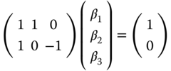
For example, if the sum of the first two coefficients must equal 1 and the first and third ones should be equal, the joint restrictions can be written as:
To estimate the constrained OLS estimator, we write the Lagrangian:
with ![]() and
and ![]() the vector of Lagrange multipliers associated to the different constraints.1 The Lagrangian can also be written as:
the vector of Lagrange multipliers associated to the different constraints.1 The Lagrangian can also be written as:
The first‐order conditions become:
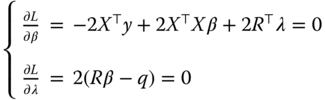
which can also be written in matrix form:
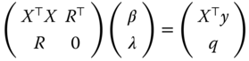
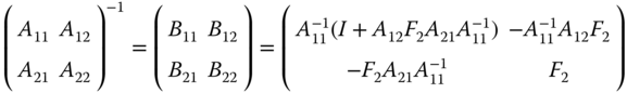
The constrained OLS estimator can be obtained using the formula for the inverse of a partitioned matrix (see equation 2.18):
with ![]() and
and ![]() .
.
We have here ![]() . The constrained estimator is then:
. The constrained estimator is then: ![]() , with
, with ![]() and
and ![]()
The unconstrained estimator being ![]() , we finally get:
, we finally get:
The difference between the constrained and the unconstrained estimators is then a linear combination of the excess of the linear constraints of the model evaluated for the unconstrained model.
3.2.3 Inter‐equations Correlation
We consider a system of ![]() equations denoted
equations denoted ![]() , with
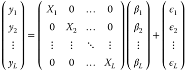
, with ![]() . In matrix form, the system can be written as follows:
. In matrix form, the system can be written as follows:
The covariance matrix of the errors of the system is:
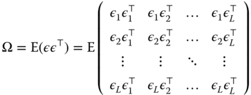
We suppose that the errors of two equations ![]() and
and ![]() for the same observations are correlated and that the covariance, denoted by
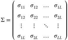
for the same observations are correlated and that the covariance, denoted by ![]() , is constant. With this hypothesis, the covariance matrix is:
, is constant. With this hypothesis, the covariance matrix is:

Denoting by ![]() the matrix of inter‐equations covariances, we have:
the matrix of inter‐equations covariances, we have:
Because of the inter‐equations correlations, the efficient estimator is the GLS estimator: ![]() . This estimator, first proposed by Zellner (1962), is known by the acronym SUR for seemingly unrelated regression. It can be obtained by applying OLS on transformed data, each variable being pre‐multiplied by
. This estimator, first proposed by Zellner (1962), is known by the acronym SUR for seemingly unrelated regression. It can be obtained by applying OLS on transformed data, each variable being pre‐multiplied by ![]() . This matrix is simply
. This matrix is simply ![]() . Denoting by
. Denoting by ![]() the elements of
the elements of ![]() , the transformed response and covariates are:
, the transformed response and covariates are:

![]() is a matrix that contains unknown parameters, which can be estimated using residuals of a consistent but inefficient preliminary estimator, like OLS. The efficient estimator is then obtained the following way:
is a matrix that contains unknown parameters, which can be estimated using residuals of a consistent but inefficient preliminary estimator, like OLS. The efficient estimator is then obtained the following way:
- first, each equation is estimated separately by OLS and we note
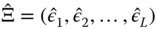 the
the  matrix for which every column is the residual vector of one of the equations in the system,
 - then, estimate the covariance matrix of the errors:
 ,
, - compute the matrix
 and use it to transform the response and the covariates of the model,
 - finally, estimate the model by applying OLS on transformed data.
![]() can conveniently be computed using the Cholesky decomposition, i.e., computing the lower‐triangular matrix
can conveniently be computed using the Cholesky decomposition, i.e., computing the lower‐triangular matrix ![]() such that
such that ![]() .
.
3.2.4 SUR With Panel Data
Applying the SUR estimator on panel data is straightforward when only the between or the within variability of the data is taken into account. In this case, one just has to apply the above formula using the variables in individual means (between‐SUR) or in deviations from individual means (within‐SUR). Taking into account both sources of variability requires more attention and leads to the SUR error component model proposed by Avery (1977) and Baltagi (1980). The errors of the model then present two sources of correlation:
- the correlation of the SUR model, i.e., inter‐equations correlation,
- the correlation taken into account in the error component model, i.e., the intra‐individual correlations.
Every observation is now characterized by three indexes: ![]() is the observation of
is the observation of ![]() for equation
for equation ![]() , individual
, individual ![]() and period
and period ![]() . The observations are first ordered by equation, then by individual. Denoting
. The observations are first ordered by equation, then by individual. Denoting ![]() the error vector for equation
the error vector for equation ![]() and individual
and individual ![]() , one gets:
, one gets:
The errors concerning different individuals being uncorrelated, the correlation matrix for two equations and all individuals is:
Finally, for the whole system of equations, denoting ![]() and
and ![]() the two matrices of dimension
the two matrices of dimension ![]() containing the parameters
containing the parameters ![]() and
and ![]() , the covariance matrix of the errors is:
, the covariance matrix of the errors is:
The SUR error component model may be obtained by applying OLS on transformed data, every variable being pre‐multiplied by ![]() .
.
and may be estimated using the Cholesky decomposition of ![]() and
and ![]() (see Kinal and Lahiri, 1990).
(see Kinal and Lahiri, 1990).
The two error covariance matrices being unknown, the error‐component SUR estimator is obtained with the following steps:
- first, each equation is estimated separately using a consistent method of estimation (for example OLS): we denote by
 and
and  the matrices of residuals in deviation from the individual means and in individual means, respectively,
 - next, we estimate the error covariance matrices:
 and
and 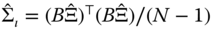 ,
, - we then compute the matrices
 and
and  and hence, through 3.8, we obtain the transformed variables
  and
and  ,
, - finally, we apply OLS on
 and
and  .
.
Different choices of preliminary estimates lead to different SUR‐error component estimators. For example, Baltagi (1980) used the method of Amemiya (1971) while Avery (1977) chose the one of Swamy and Arora (1972).
3.3 The Maximum Likelihood Estimator
An alternative to the OLS estimator presented in the previous chapter is the maximum likelihood estimator. Contrary to the GLS estimator, the parameters are not estimated sequentially (first ![]() and then
and then ![]() ) but simultaneously.
) but simultaneously.
3.3.1 Derivation of the Likelihood Function
In order to write the likelihood of the model, the distribution of the errors must be perfectly characterized; compared with the GLS model, we then must add an hypothesis concerning the distribution of the two components of the error term, the individual ![]() and the idiosyncratic
and the idiosyncratic ![]() effects: we'll suppose that they are both normally distributed. The likelihood is the joint density for the whole sample, which is the product of the individual densities in the case of a random sample. This is not the case here, as the
effects: we'll suppose that they are both normally distributed. The likelihood is the joint density for the whole sample, which is the product of the individual densities in the case of a random sample. This is not the case here, as the ![]() observations of individual
observations of individual ![]() are correlated because of the common individual effect. The model to be estimated is then:
are correlated because of the common individual effect. The model to be estimated is then:
with ![]() and
and ![]() . For a given value of the individual effect,
. For a given value of the individual effect, ![]() , the density for
, the density for ![]() is:
is:

For a given value of ![]() , the distribution of
, the distribution of ![]() is the one of a vector of independent random deviates, and the joint distribution is therefore the product of individual densities:
is the one of a vector of independent random deviates, and the joint distribution is therefore the product of individual densities:

The unconditional distribution is obtained by integrating out the individual effects ![]() , which means that the mean value of the density is computed for all possible values of
, which means that the mean value of the density is computed for all possible values of ![]() :
:

with, denoting ![]() ,
, ![]() and
and ![]() :
:
Denoting by ![]() the first term, we have
the first term, we have ![]() and the joint density is then (denoting
and the joint density is then (denoting ![]() ):
):
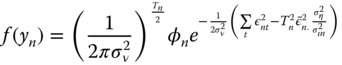
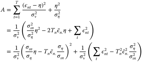
For the second term, we have:

so that the joint density for an individual is finally:
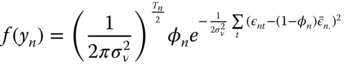
The contribution of the ![]() ‐th individual to the log likelihood function is simply the logarithm of the joint density:
‐th individual to the log likelihood function is simply the logarithm of the joint density:

The log likelihood function is then obtained by summing over all the individuals of the panel:

or, more simply in the special case of a balanced panel:

Note also that:
3.3.2 Computation of the Estimator
The first derivatives of the log likelihood are, denoting ![]() :
:
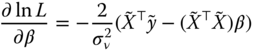


Solving 3.9, we obtain:
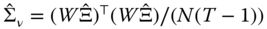
The estimator of ![]() is simply obtained by using 3.10 as the residual variance of the model estimated on the transformed data:
is simply obtained by using 3.10 as the residual variance of the model estimated on the transformed data:

Finally, using 3.11 and 3.13, the transformation parameter is:

The estimation can be performed iteratively. Starting from an estimator of ![]() (for example the within estimator), we calculate
(for example the within estimator), we calculate ![]() using the formula given by 3.14. We then transform the response and the covariates using this estimator of
using the formula given by 3.14. We then transform the response and the covariates using this estimator of ![]() and we compute a second estimation of
and we compute a second estimation of ![]() using 3.12. These computations are repeated until the convergence of
using 3.12. These computations are repeated until the convergence of ![]() and
and ![]() .
. ![]() is then estimated using 3.13.
is then estimated using 3.13.
3.4 The Nested Error Components Model
3.4.1 Presentation of the Model
The nested random effect model is relevant when the individuals can be put together in different groups. For example, with a panel of firms, groups may be constituted by regions or production sectors.
In this chapter, we'll restrict ourselves to panels with two characteristics:
- panels without time effects,
- balanced panels inside each group, which means that, for every group, the number of observations for each individual is the same.
The number of individuals and the length of time series for two groups may be different. This is why this model, presented in Baltagi et al. (2001) is called the unbalanced nested error component model, even if its unbalancedness must be understood in the very restrictive sense we've just described.
Three effects will now be considered: the usual individual ![]() and idiosyncratic
and idiosyncratic ![]() effects, but also a new one that represents group effects
effects, but also a new one that represents group effects ![]() . Denoting by
. Denoting by ![]() the matrix of group dummies:
the matrix of group dummies:
![]() is block‐diagonal with
is block‐diagonal with ![]() (the number of groups) blocks of the following shape:
(the number of groups) blocks of the following shape:
Replacing ![]() by
by ![]() and
and ![]() by
by ![]() , this can be rewritten as a linear combination of three symmetric, idempotent, and orthogonal matrices which sum to
, this can be rewritten as a linear combination of three symmetric, idempotent, and orthogonal matrices which sum to ![]() :
:
where:
 is the within‐individual transformation,
 is the between‐individual transformation measured as a difference with the group mean,
 is the between‐group transformation.
This expression enables to easily find the expression for ![]() , denoting
, denoting ![]() and
and ![]() :
:
which finally writes:
with ![]() and
and ![]() .
.
The model can therefore be estimated by OLS on transformed variables for which part of the individual and the group mean (respectively ![]() and
and ![]() have been subtracted).
have been subtracted).
3.4.2 Estimation of the Variance of the Error Components
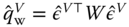
We proceed along the lines of section 3.1.3. Using residuals from a preliminary estimation ![]() denoted
denoted ![]() , we compute a quadratic form of
, we compute a quadratic form of ![]() with a matrix
with a matrix ![]()
![]() .
.
Replacing ![]() by its expression and denoting
by its expression and denoting ![]() , we obtain:
, we obtain:
or, denoting ![]() :
:

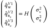
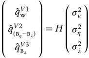
The most popular estimators are obtained by computing the three quadratic forms with the within‐individual, between‐individual and between‐group matrices. We then get the following system of equations:
with:

Using the following results:
![]() ,
, ![]() ,
, ![]() ,
, ![]() ,
, ![]() ,
, ![]() ,
, ![]() ,
, ![]() ,
, ![]() ,
, ![]() ,
, ![]() ,
, ![]() ,
, ![]() ,
, ![]() ,
, ![]() ,
, ![]() ,
, ![]() ,
, ![]() ,
, ![]() .
.
We finally obtain:
or:

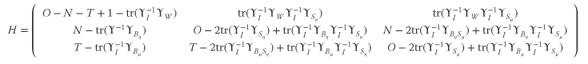
Baltagi et al. (2001) have proposed a variant of the Amemiya (1971) estimator (where the within estimator is used for the three quadratic forms), the Wallace and Hussain (1969) estimator (the OLS estimator is used for the three quadratic forms) and of the Swamy and Arora (1972) estimator (the within, between‐individual and between‐group are used respectively for the within, between‐individual, and between‐group quadratic forms). The detailed formulas are presented in Figure 3.2.
Amemiya (1971):
Wallace and Hussain (1969):

Swamy and Arora (1972):

Figure 3.2Error components estimators for the nested error component model.