
Chapter 9
Count Data and Limited Dependent Variables
It is often the case in economics that the dependent variable is not continuous so that OLS estimation is not appropriate. On the one hand, the response may be a count, i.e., it takes only non‐negative integer values. In this case, the most commonly used specifications are the Poisson and the NegBin models. On the other hand, the response may exhibit limited dependence. In this case, one can assume that there exists a continuous non‐observable variable called ![]() . The value of
. The value of ![]() is not observed for some part of the domain or not observed at all. The different cases are depicted in Figure 9.1:
is not observed for some part of the domain or not observed at all. The different cases are depicted in Figure 9.1:
- Figure 9.1a presents the case of a binomial variable (
 ), which indicates the position of
  relative to a threshold
  ,
, - Figure 9.1b presents the case of an ordinal variable (
 ), which indicates the position of
  relative to two thresholds
  and
and  ,
, - Figure 9.1c presents the case of a left‐ truncated variable at
 ; on the right of
  , we have
  , observations characterized by
  are simply not available,
 - Figure 9.1d presents the case of a left‐censored variable at
 ; as for the truncated case, one observes, on the right of
  ,
,  . The sample contains observations for which
  , but the corresponding values of
  are unobserved.

Figure 9.1Limited dependent variable.
Some of these models belong to a broad category called “generalized linear models”. More specifically, this concerns:
- the binomial model and especially two particular cases, the logit and the probit models,
- the Poisson model.
The Negbin model is also a generalized linear model if its supplementary parameter is a fixed parameter and is not estimated.
In a cross‐section context, both base R and several packages provide the relevant estimators, using the maximum likelihood method:
- probit, logit and Poisson models can be fitted using the
glmfunction, - the NegBin model can be estimated using the
glm.nbfunction of the MASS package, - the ordinal model can be fitted using the
polrfunction of this same package, - the censored model can be estimated using the
tobitfunction of the AER package or thecensRegfunction of the censReg package, - the truncated model can be fitted using the
truncregfunction of the truncreg package.
The pglm package provides similar estimators for panel data. It enables the estimation of binomial and Poisson models and for convenience, also for Negbin and ordinal models, even if strictly speaking these last two are not proper generalized linear models.
The pldv function of the plm package provides panel estimators for the case where the response is either truncated or censored.
These models are often estimated using the maximum likelihood method, which requires to make strong hypotheses concerning the distribution of the response. When these hypotheses are not valid, except for very special cases, the estimator is no longer consistent.
This last is a very general drawback of maximum likelihood estimators, but there is also another drawback that is specific to panel data. In linear models, individual effects can be removed using an appropriate transformation (within or first differences) or can be directly estimated. This is not the case for most of the models presented in this chapter; the individual effects cannot be removed, and their estimation leads to the incidental parameter problem.
When ![]() for fixed
for fixed ![]() , for the linear model, the estimation of individual effects is not consistent, as the number of parameters to be estimated grows with
, for the linear model, the estimation of individual effects is not consistent, as the number of parameters to be estimated grows with ![]() and the variance of the estimators is constant. On the contrary, nevertheless, the estimator of the vector of parameters of interest
and the variance of the estimators is constant. On the contrary, nevertheless, the estimator of the vector of parameters of interest ![]() is consistent.
is consistent.
Differently from the linear case, for most of the models reviewed in this chapter, when the individual effects are estimated, their inconsistency “contaminates” the estimation of ![]() , which becomes inconsistent as well1. This incidental parameter problem leads to abandoning the fixed effects models where the fixed effects are estimated in favor of three alternatives2:
, which becomes inconsistent as well1. This incidental parameter problem leads to abandoning the fixed effects models where the fixed effects are estimated in favor of three alternatives2:
- the random effects model, which is always usable: one first writes the individual effects' conditional probabilities and then computes the unconditional probabilities by integrating out the individual effects, making a hypothesis about their distribution,
- a fixed effects model, which uses the notion of sufficient statistic: for example, in a logit model, the probability of being unemployed at period
 depends on the individual effect, and so does the number of spells of unemployment for every period. By contrast, the ratio of this probability, which is the probability to be unemployed in period
  knowing the total number of periods for which the individual is unemployed, does not contain the individual effect. This technique, which is not available for all the models reviewed, enables, like the within transformation of the linear models, to get rid of the individual effects,
 - for censored or truncated responses, the linear model can be consistently applied if some observations are removed from the sample beforehand (one then speaks of a trimmed estimator).
In the next sections, we will present the three categories of models previously cited: binomial and ordinal models, truncated and censored models, and count data models. For each of these three sections, we will first briefly describe the estimators used with cross‐sectional data. We will then present the estimators appropriate for panel data. We will finally reproduce different empirical examples of these models.
9.1 Binomial and Ordinal Models
9.1.1 Introduction
9.1.1.1 The Binomial Model
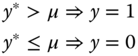
We consider a model for which the response is binomial, and we denote without loss of generality the two possible values 0 and 1. We then define a latent variable ![]() that is continuous on the real line and is unobserved. The latent variable is linked to the observable binomial variable
that is continuous on the real line and is unobserved. The latent variable is linked to the observable binomial variable ![]() by the following rule of observation:
by the following rule of observation:
The value of the latent variable is the sum of a linear combination of the covariates and an error term. Without loss of generality, if ![]() includes an intercept, we set
includes an intercept, we set ![]() .
.
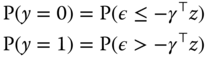
The variance of ![]() is not identified; it can therefore be set to 1 or to any other arbitrary value. Probabilities for the two possible values of the response are then:
is not identified; it can therefore be set to 1 or to any other arbitrary value. Probabilities for the two possible values of the response are then:
Denoting by ![]() the cumulative density of
the cumulative density of ![]() , we then have:
, we then have:
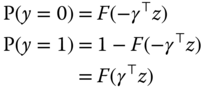
the last expression being valid if the density of ![]() is symmetric. Denoting
is symmetric. Denoting ![]() , which equals
, which equals ![]() for
for ![]() , the probability of the outcome can be expressed in a compact form:
, the probability of the outcome can be expressed in a compact form:
Two distributions are often used: the normal distribution:
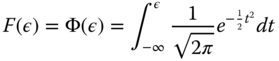
which leads to the probit model, and the logistic distribution:
which leads to the logit model.
For a sample of size ![]() , the log‐likelihood function is obtained by summing the logs of (9.1) for all the observations:
, the log‐likelihood function is obtained by summing the logs of (9.1) for all the observations:

9.1.1.2 Ordered Models
An ordered model is a model for which the response can take ![]() distinct values (with
distinct values (with ![]() ). The construction of the model is very similar to the one of the binomial model. We consider a latent variable, like before equal to the sum of a linear combination of the covariates and an error:
). The construction of the model is very similar to the one of the binomial model. We consider a latent variable, like before equal to the sum of a linear combination of the covariates and an error:
Denoting ![]() a vector of parameters, with
a vector of parameters, with ![]() and
and ![]() , the rule of observation for the different values of
, the rule of observation for the different values of ![]() is then:
is then:

Denoting by ![]() the cumulative density of
the cumulative density of ![]() , the probability for a given value
, the probability for a given value ![]() of
of ![]() is:
is:
The probability of the outcome can be written:
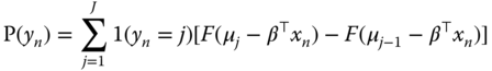
For a sample of size ![]() , the log‐likelihood function is obtained by summing the logarithms of (9.2) for all the observations:
, the log‐likelihood function is obtained by summing the logarithms of (9.2) for all the observations:

As for the binomial model, the most common choices for the distribution of ![]() are the normal and the logistic distributions, which lead respectively to the ordered probit and logit models.
are the normal and the logistic distributions, which lead respectively to the ordered probit and logit models.
9.1.2 The Random Effects Model
For panel data, we now have repeated observations of ![]() for the same individuals. The latent variable is then defined by:
for the same individuals. The latent variable is then defined by:
We assume as usual that the error can be written as the sum of an individual effect ![]() and an idiosyncratic term
and an idiosyncratic term ![]() . Two observations for the same individual are then correlated because of the common term
. Two observations for the same individual are then correlated because of the common term ![]() . If the
. If the ![]() vector contains an intercept, we can suppose, without loss of generality, that
vector contains an intercept, we can suppose, without loss of generality, that ![]() .
.
9.1.2.1 The Binomial Model
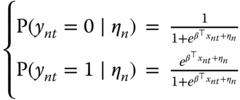
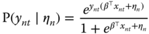
For a given value of ![]() , the probability of the outcome for individual
, the probability of the outcome for individual ![]() at period
at period ![]() is defined as before:
is defined as before:
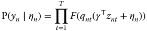
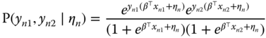
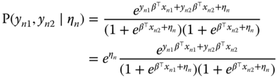
Denoting ![]() , the joint probability for all the periods for individual
, the joint probability for all the periods for individual ![]() is:
is:
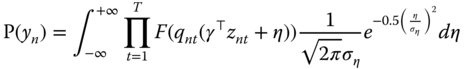
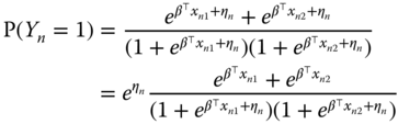
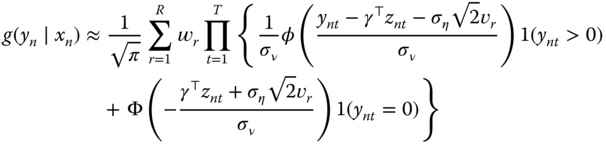
The unconditional probability is obtained by integrating out this expression for ![]() . Assuming that the distribution of
. Assuming that the distribution of ![]() is normal with a standard deviation of
is normal with a standard deviation of ![]() , we obtain:
, we obtain:
With the change of variable:
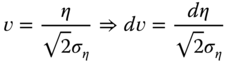
we obtain

There is no closed‐form for this integrand, but it can be efficiently numerically approximated using Gauss‐Hermite quadrature. This method consists in evaluating the function for different values of ![]() (denoted
(denoted ![]() ) and computing a linear combination of these evaluations, with weights denoted by
) and computing a linear combination of these evaluations, with weights denoted by ![]() . For a fixed number of evaluations
. For a fixed number of evaluations ![]() , the values of
, the values of ![]() are tabulated.
are tabulated.
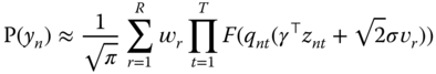
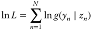
and the log‐likelihood function is obtained by summing over all the individuals the logarithm of (9.3).
9.1.2.2 Ordered Models
The line of reasoning is very similar to that of binomial models. The joint probability for an individual ![]() for a given value of the individual effect is:
for a given value of the individual effect is:

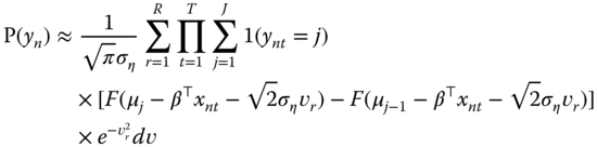
Assuming a normal distribution for the individual effects, the unconditional probability is:

Using the same change of variable as previously, we obtain:
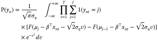
which can be approximated using Gauss‐Hermite quadrature:
9.1.3 The Conditional Logit Model
The random effects model is consistent only if the individual effects are uncorrelated with the covariates. If it is not the case, the conditional logit model can be used. It is well known in the statistic literature and has been introduced in panel data econometrics by Chamberlain (1980).
The general presentation of this model is quite complex, but the intuition of it can be perceived using the special case where ![]() . We denote
. We denote ![]() . Only the individuals for which
. Only the individuals for which ![]() can be used to estimate the conditional logit model (more generally, only individuals for which
can be used to estimate the conditional logit model (more generally, only individuals for which ![]() may be used).
may be used).
For a given period ![]() , the probabilities for the two values of
, the probabilities for the two values of ![]() are:
are:
or more generally:
If the idiosyncratic components of the errors are i.i.d., the joint probability for two observations is simply the product of ![]() and
and ![]() :
:
or also, as one and only one of the two ![]() equals 1:
equals 1:
 (9.4)
(9.4)
The probability that ![]() is equal to the sum of the probabilities of:
is equal to the sum of the probabilities of:
 and
and  , which is
  ,
, and
and  , which is
  .
.
which is therefore:
Dividing (9.4) by (9.5), one finally obtains the joint probability of ![]() and
and ![]() given their sum:
given their sum:

This conditional probability is free of the individual effect and the likelihood that uses this expression can therefore be considered as a fixed effects logit model. Note that there is no similar estimator for the probit model.
9.2 Censored or Truncated Dependent Variable
9.2.1 Introduction
It's often the case in economics that the response is only observed on a certain range of values; we then say that the dependent variable is truncated. For example:
- if the response is a proportion, it is necessarily left‐ truncated on 0 and right‐truncated on 1,
- consumption for a good is necessarily positive and therefore left‐truncated on 0,
- the demand for a sports event is necessarily lower or equal to the number of seats in the stadium and is therefore right‐ truncated to this capacity.
From now on, we will consider the most common case, which is a 0 left truncation, but the models we will present easily extend to the case of left or/and right truncations at any value.
As usual, we will assume that the dependent variable can be represented by a latent variable ![]() that equals the sum of a linear combination of different covariates and an error term.
that equals the sum of a linear combination of different covariates and an error term.
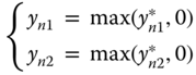
The observed response ![]() equals
equals ![]() if it is not in the truncated zone (i.e., here, if it's strictly positive) and equals the truncature (here, 0) otherwise.
if it is not in the truncated zone (i.e., here, if it's strictly positive) and equals the truncature (here, 0) otherwise.
Two kinds of samples can be used to estimate this model:
- a sample is truncated when only observations for which
 are available (we therefore don't even know the values of the covariates
  for observations for which
  is in the truncation zone),
 - a sample is censored when it consists of observations for which
 is either inside or outside the truncation zone.
This latter case is particularly important in econometrics and leads to a model which is called the tobit model (Tobin, 1958). From now, we'll refer to the truncated model when the first kind of sample is used and to the censored model for the second kind of sample.
We'll first analyze why applying a linear regression to a censored or a truncated model leads to inconsistent estimators. We'll then present a non‐parametric method that leads, removing some specific observations, to a consistent estimator while making minimal hypotheses on the model errors. We'll conclude this section with the maximum likelihood estimator, which relies on the much stronger hypothesis of homoscedasticity and normal distribution.
9.2.2 The Ordinary Least Squares Estimator
Let ![]() be the density of the distribution of
be the density of the distribution of ![]() which is supposed, without loss of generality as long as the equation contains an intercept, to be of 0 expected value. We then have:
which is supposed, without loss of generality as long as the equation contains an intercept, to be of 0 expected value. We then have:
If ![]() were observed, OLS would be a consistent estimator for
were observed, OLS would be a consistent estimator for ![]() . This is not the case when we only observe the truncated variable
. This is not the case when we only observe the truncated variable ![]() . On the truncated sample, we have
. On the truncated sample, we have ![]() , or
, or ![]() . The distribution of
. The distribution of ![]() for the sample is then
for the sample is then ![]() , depicted by the dotted line in Figure 9.2.
, depicted by the dotted line in Figure 9.2.

Figure 9.2Distribution of  and
and  .
.
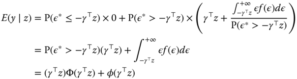
The distribution of ![]() is not symmetric around 0, and its expected value is positive, because the left side of the distribution, corresponding to values of
is not symmetric around 0, and its expected value is positive, because the left side of the distribution, corresponding to values of ![]() , is truncated. We therefore have:
, is truncated. We therefore have:
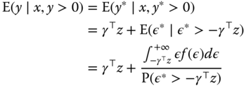
which is, for a normal distribution:
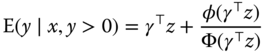
or, subtracting ![]() :
:
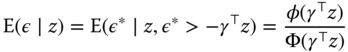
![]() is known as the inverse mills ratio and is a decreasing function of its argument. Computing the derivative with respect to one covariate
is known as the inverse mills ratio and is a decreasing function of its argument. Computing the derivative with respect to one covariate ![]() , we obtain:
, we obtain:
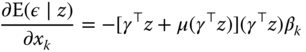
which is negative if ![]() , as
, as ![]() is the average of
is the average of ![]() for
for ![]() and is therefore greater than
and is therefore greater than ![]() . The OLS estimator computed on the truncated sample is therefore downward biased.
. The OLS estimator computed on the truncated sample is therefore downward biased.
For the censored sample, we have ![]() for censored observations. We then have:
for censored observations. We then have:
where the last expression holds for a normal distribution. Subtracting ![]() , we obtain the expected value of the error of the censored model:
, we obtain the expected value of the error of the censored model:
Computing once again the derivative with respect to a covariate ![]() , we have:
, we have:
which, as previously, has the opposite sign of ![]() , implying that the OLS estimator on the censored sample is downward biased.
, implying that the OLS estimator on the censored sample is downward biased.
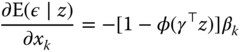
The bias of the OLS estimator on censored and truncated samples is illustrated on Figure 9.3
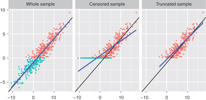
Figure 9.3OLS bias for the censored and the truncated samples.
9.2.3 The Symmetrical Trimmed Estimator
The OLS estimator is inconsistent because the truncation leads to an asymmetric distribution for the errors, for which the expected values depends on ![]() . Powell (1986) proposes to restore the symmetry by removing some observations.
. Powell (1986) proposes to restore the symmetry by removing some observations.
9.2.3.1 Truncated Sample
In the case of the truncated sample, observations for which ![]() , or
, or ![]() , are missing. The symmetry may be restored by removing from the right side of the distribution, the observations for which
, are missing. The symmetry may be restored by removing from the right side of the distribution, the observations for which ![]() , or
, or ![]() . The distributions of
. The distributions of ![]() and
and ![]() are depicted by the dashed line in Figure 9.2. In this case, we have:
are depicted by the dashed line in Figure 9.2. In this case, we have:
A consistent estimator may be obtained using the normal conditions and restricting the sample to observations for which ![]() . Denoting by
. Denoting by ![]() the function that is equal to 1 if
the function that is equal to 1 if ![]() is true and 0 otherwise, we have:
is true and 0 otherwise, we have:

These first‐order conditions may be obtained by minimizing the function:

In this case, all the observations for which ![]() and those for which
and those for which ![]() have a weight equal to
have a weight equal to ![]() in the objective function and a zero weight in the first‐order conditions. The weight in the objective function ensures that fallacious solutions of the first‐order conditions like
in the objective function and a zero weight in the first‐order conditions. The weight in the objective function ensures that fallacious solutions of the first‐order conditions like ![]() are excluded.
are excluded.
9.2.3.2 Censored Sample
In the case of the censored sample, symmetry is restored by replacing ![]() by
by ![]() when
when ![]() (as
(as ![]() is replaced by 0 when
is replaced by 0 when ![]() ). We then have:
). We then have:

These first‐order conditions may be obtained by minimizing the following function:
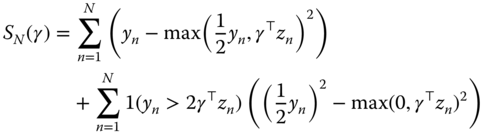
Observations for which ![]() now have a weight equal to
now have a weight equal to ![]() in the objective function and a zero weight in the first‐order conditions.
in the objective function and a zero weight in the first‐order conditions.
9.2.4 The Maximum Likelihood Estimator
If we can assume that the errors are normal and homoscedastic, a more efficient estimator is the maximum likelihood estimator.
9.2.4.1 Truncated Sample
The maximum likelihood estimator for a truncated sample has been proposed by Hansman and Wise (1976). The density of the distribution of ![]() is normal, with expected value equal to
is normal, with expected value equal to ![]() and standard deviation
and standard deviation ![]() . We then have:
. We then have:

The probability of ![]() being negative is:
being negative is: ![]() .
.
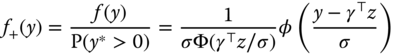
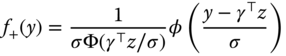
The density of the distribution of ![]() , denoted
, denoted ![]() , is the zero left‐truncated distribution of
, is the zero left‐truncated distribution of ![]() : We then have:
: We then have:
The log‐likelihood function is obtained by summing the logarithms of the density (9.13) for the ![]() observations in the sample:
observations in the sample:

9.2.4.2 Censored Sample
When the sample is censored, the distribution of ![]() is a mix of a discrete and a continuous distribution. An observation for which
is a mix of a discrete and a continuous distribution. An observation for which ![]() enters the log‐likelihood function as:
enters the log‐likelihood function as:

while for a positive observation, the contribution to the likelihood is the truncated normal density:
times the probability that ![]() be positive:
be positive: ![]() . We finally get the log‐likelihood function (9.15):
. We finally get the log‐likelihood function (9.15):

9.2.5 Fixed Effects Model
Honoré (1992) proposed a symmetrical trimmed estimator that is an extension of Powell (1986)'s estimator to panel data. For now, we consider a panel with only two observations for every individual and one covariate.
The only hypothesis made concerning the errors ![]() and
and ![]() is that they are identically distributed. The symmetry hypothesis, which was required for the Powell (1986) estimator to be consistent, is not necessary here.
is that they are identically distributed. The symmetry hypothesis, which was required for the Powell (1986) estimator to be consistent, is not necessary here.
9.2.5.1 Truncated Sample
For the truncated model, only observations for which ![]() are available. Figure 9.43 presents the distribution of
are available. Figure 9.43 presents the distribution of ![]() and
and ![]() .
.
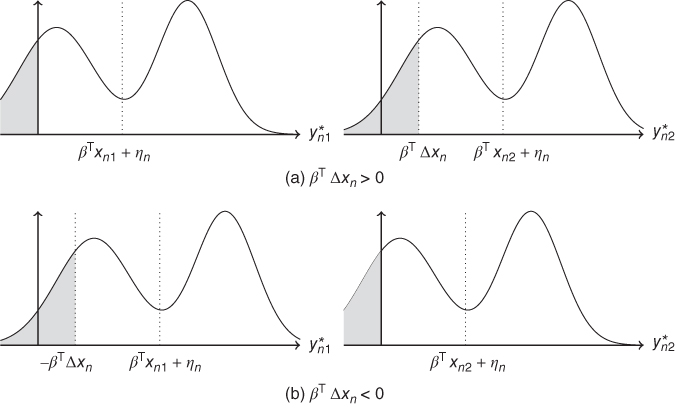
Figure 9.4Distribution of  and of
  .
.
With the hypotheses we've made, these two distributions only differ by their position, ![]() being centered on
being centered on ![]() and
and ![]() on
on ![]() . Because of the truncation, the two distributions conditioned to the fact that the observation is in the sample (
. Because of the truncation, the two distributions conditioned to the fact that the observation is in the sample (![]() ), to the values of the covariates (
), to the values of the covariates (![]() ) and to that of the individual effect (
) and to that of the individual effect (![]() ) are more substantially different. If
) are more substantially different. If ![]() (Figure 9.4a), the truncated part of the distribution of
(Figure 9.4a), the truncated part of the distribution of ![]() is larger than the one of
is larger than the one of ![]() . However, identical distributions can be obtained by truncating
. However, identical distributions can be obtained by truncating ![]() not at 0 (which is the selection rule of the sample) but at
not at 0 (which is the selection rule of the sample) but at ![]() . In the case where
. In the case where ![]() (Figure 9.4b),
(Figure 9.4b), ![]() is similarly truncated at
is similarly truncated at ![]() .
.
We then obtain two identical conditional distributions for:
 and
and  in the case when
  ,
, and
and  in the case when
  ,
,
More generally, the observations that should be removed to restore symmetry are those for which ![]() or
or ![]() . This situation is depicted in Figure 9.5. When
. This situation is depicted in Figure 9.5. When ![]() (9.5a), the joint distribution of
(9.5a), the joint distribution of ![]() is symmetric around the
is symmetric around the ![]() line which is the
line which is the ![]() line with intercept
line with intercept ![]() . Truncating at
. Truncating at ![]() and
and ![]() , we obtain two symmetric zones
, we obtain two symmetric zones ![]() and
and ![]() . The probability of having
. The probability of having ![]() in zones
in zones ![]() or
or ![]() is the same. This result leads to a first‐moment condition:
is the same. This result leads to a first‐moment condition:
Moreover, by symmetry, in Figure 9.5a:
- the vertical distance between
 in zone
  on the
  line is
  ,
, - the horizontal distance between
 in
in  and the
  line is
  ,
,
which can be written as a second‐moment condition:
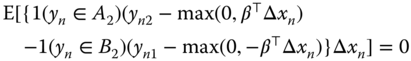
For a sample of size ![]() , truncated as previously described, the sample analogues of the two moment conditions (9.16) and (9.17) are:
, truncated as previously described, the sample analogues of the two moment conditions (9.16) and (9.17) are:
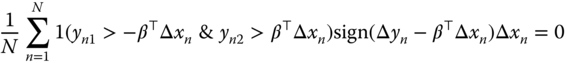

(9.18 and 9.19) are respectively the first‐order conditions of the LAD and of the least squares estimator. These first‐order conditions may be obtained by maximizing:
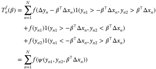
with:

If ![]() , we obtain the trimmed least squares estimator; if
, we obtain the trimmed least squares estimator; if ![]() , we obtain the trimmed least absolute deviations estimator. Only the observations for which
, we obtain the trimmed least absolute deviations estimator. Only the observations for which ![]() are included in the first‐order conditions, the presence of
are included in the first‐order conditions, the presence of ![]() in the objective function excluding trivial solutions.
in the objective function excluding trivial solutions.
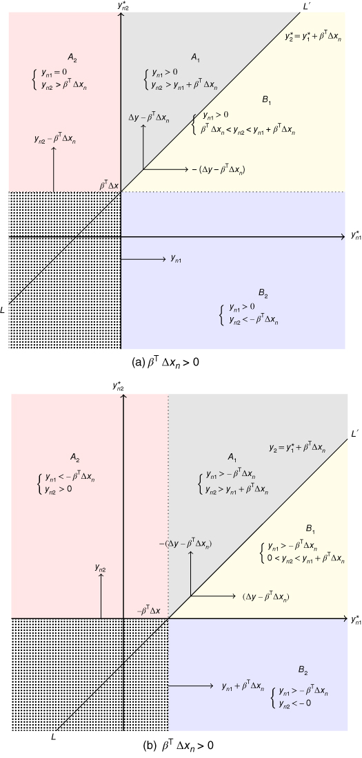
Figure 9.5Symmetry of the distribution of  .
.
9.2.5.2 Censored Sample
For the censored sample, observations for which ![]() are available, the observation rule for
are available, the observation rule for ![]() being:
being:
From Figure 9.5, we can see that not only ![]() and
and ![]() are symmetrical but also
are symmetrical but also ![]() defined by
defined by ![]() and
and ![]() defined by
defined by ![]() .
.
Therefore, to restore symmetry for the censored sample, we have to get rid of the zone for which ![]() and
and ![]() (the dotted zone on Figure 9.5).
(the dotted zone on Figure 9.5).
The symmetry between ![]() and
and ![]() leads to the following moment condition:
leads to the following moment condition:
Moreover, for:
 in
in  , the vertical distance to the limit of the zone is
  ,
, in
in  , the horizontal distance to the limit of the zone is
which translates into the following moment condition:
Using (9.16 and 9.20), we obtain:
and using (9.17 et 9.21), we obtain:
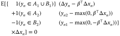
The sample analogues to (9.22) are the first‐order conditions of the following function:
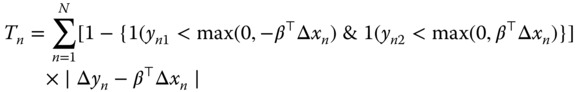
which is the trimmed LAD estimator on the censored sample.
Finally, the sample equivalent of (9.23) are the first‐ order conditions of the following function:
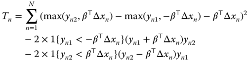
which is the trimmed least squares estimator for the censored sample. The trimmed LAD and least squares estimators have been extended to the case where the dependent variable is two‐sided censored or truncated by Alan et al. (2013).
9.2.6 The Random Effects Model
The trimmed estimator has two useful features: it is robust to non‐normality and heteroscedasticity, on the one hand, and to correlation between the individual effects and the covariates, on the other hand, the individual effects being wiped out by the first‐ difference transformation. However, if the errors are normal and homoscedastic and if the individual effects are also normal and uncorrelated with the covariates, the maximum likelihood estimator is consistent and more efficient.
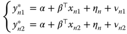
For panel data with individual effects, the latent variable writes:
9.2.6.1 Truncated Sample
The density of ![]() is:
is:
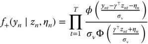
The joint density of ![]() is, assuming the independence of the errors:
is, assuming the independence of the errors:
Assuming that the distribution of individual effects is normal with a standard deviation equal to ![]() , the unconditional joint density is obtained by integrating out (9.26) for the individual effects:
, the unconditional joint density is obtained by integrating out (9.26) for the individual effects:
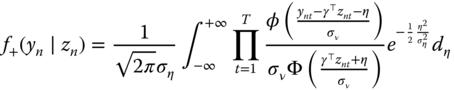
Using the change of variable ![]() , we obtain:
, we obtain:

which can be approximated by the Gauss‐Hermite quadrature method:
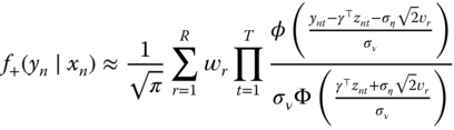
The log‐likelihood function for the truncated model is then simply obtained by summing the logarithms of (9.29) for all individuals:

9.2.6.2 Censored Sample
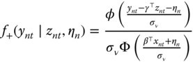
In this case, the conditional distribution of ![]() is either given by a probability or by a density:
is either given by a probability or by a density:

Using a similar reasoning as for the truncated model, individual ![]() contributes to the likelihood with a product of probabilities and/or densities:
contributes to the likelihood with a product of probabilities and/or densities:
The log‐likelihood function for the censored sample is obtained by summing over all the individuals the logarithm of (9.31):
9.3 Count Data
We now consider the case where the response is a count. We will first briefly review the estimation of count data models in a cross‐sectional context, and then we will describe specific estimators for panel data.
9.3.1 Introduction
The two most widely used models when the response is a count are the Poisson and the NegBin models.
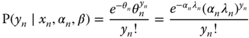
9.3.1.1 The Poisson Model
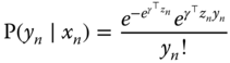
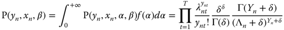
We first suppose that the response follows a Poisson distribution of parameter ![]() (which is the mean and the variance of the variable). Under this distributional assumption, the probability of observing a value
(which is the mean and the variance of the variable). Under this distributional assumption, the probability of observing a value ![]() is:
is:

Using the logarithmic link, the Poisson parameter is the exponential of the linear predictor:
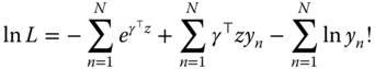
which leads to the following probability for observation ![]() :
:
Taking the logarithm of this probability and summing over all individuals, we obtain the following log‐likelihood function:
9.3.1.2 The NegBin Model
Count data often exhibit excess dispersion, i.e., the variance is greater than the mean. In this case, the NegBin model is more appropriate than the Poisson model.
Suppose that ![]() is a random variable that follows a Poisson distribution of parameter
is a random variable that follows a Poisson distribution of parameter ![]() (with
(with ![]() in the case of a logarithmic link),
in the case of a logarithmic link), ![]() being a random variable.
being a random variable.
The conditional probability of ![]() is:
is:
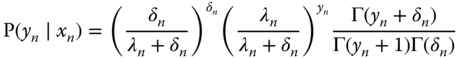
Let now suppose that ![]() follows a gamma distribution. If
follows a gamma distribution. If ![]() contains an intercept, the mean of
contains an intercept, the mean of ![]() is not identified and therefore a one‐parameter distribution, which imposes a unit mean, is chosen.
is not identified and therefore a one‐parameter distribution, which imposes a unit mean, is chosen.

Integrating out this conditional probability using the density of ![]() , we obtain:
, we obtain:

To understand the meaning of ![]() , the first two moments of
, the first two moments of ![]() are computed. For a given value of
are computed. For a given value of ![]() , we have, as for the Poisson model:
, we have, as for the Poisson model: ![]() . The unconditional mean is
. The unconditional mean is ![]() , because the expected value of
, because the expected value of ![]() equals 1.
equals 1.
To compute the unconditional variance, the variance decomposition formula is applied:
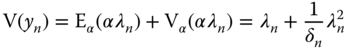
A general formula for ![]() is:
is:

For ![]() , we get the Negbin1 model, with
, we get the Negbin1 model, with ![]() and
and ![]() . In this case, the variance is proportional to the mean.
. In this case, the variance is proportional to the mean.
For ![]() , we obtain the Negbin2 model, with
, we obtain the Negbin2 model, with ![]() and
and ![]() ; here, the variance is a quadratic function of the mean.
; here, the variance is a quadratic function of the mean.
9.3.2 Fixed Effects Model
Fixed effects Poisson and NegBin models are proposed by Hausman et al. (1984).
9.3.2.1 The Poisson Model
The fixed effects Poisson model is very specific, as it doesn't suffer from the incidental parameter problem and can therefore be obtained either by estimating the individual effects or by using a sufficient statistic4.
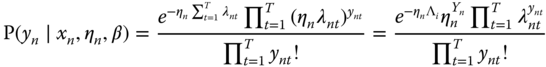
In a panel context, the Poisson parameter for individual ![]() in period
in period ![]() is written:
is written:
which means that the individual effect is multiplicative. For a given value of the individual effect, the probability of observing ![]() is:
is:

Let ![]() be the sum of all the values of the response for individual
be the sum of all the values of the response for individual ![]() and
and ![]() the sum of the Poisson parameters. A sum of Poisson variables follows a Poisson distribution with parameter equal to the sum of the parameters of the summed variables. We therefore have:
the sum of the Poisson parameters. A sum of Poisson variables follows a Poisson distribution with parameter equal to the sum of the parameters of the summed variables. We therefore have:

Let ![]() be the vector of values of
be the vector of values of ![]() for individual
for individual ![]() . We then have:
. We then have:
Applying Bayes' theorem, we obtain:
i.e., the joint probability of the components of ![]() is the product of the conditional probability of
is the product of the conditional probability of ![]() given
given ![]() and the marginal distribution of
and the marginal distribution of ![]() . This conditional probability is:
. This conditional probability is:

which implies:

As for the logit model, ![]() is a sufficient statistic, which means that it allows to get rid of the individual effects. Taking the logarithm of this expression and summing over all individuals, we obtain the within Poisson model:
is a sufficient statistic, which means that it allows to get rid of the individual effects. Taking the logarithm of this expression and summing over all individuals, we obtain the within Poisson model:
or:

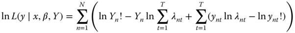
As stated previously, the Poisson model is not affected by the incidental parameter problem, as the same estimator may be obtained by estimating the individual effects. To show this result, we take the logarithm of the joint probability for the ![]() observations of
observations of ![]() for individual
for individual ![]() (equation 9.34), in order to obtain the log‐likelihood function:
(equation 9.34), in order to obtain the log‐likelihood function:
The first‐order condition for ![]() to maximize the log‐ likelihood function is:
to maximize the log‐ likelihood function is:
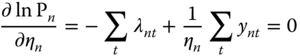
which implies that: ![]() .
.
Introducing this expression in (9.38) and summing over all ![]() , we obtain the concentrated log‐likelihood function:
, we obtain the concentrated log‐likelihood function:
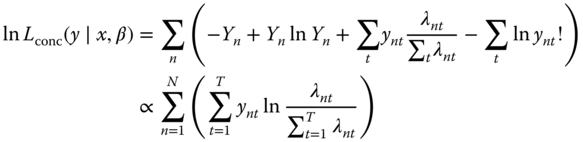
The two log‐likelihood functions (9.37) and (9.39) are proportional, they therefore lead to the same estimators of ![]() . Moreover, if a logarithmic link is chosen, we have:
. Moreover, if a logarithmic link is chosen, we have: ![]() . The likelihood is in this case proportional to:
. The likelihood is in this case proportional to:

which is similar to the likelihood of a multinomial logit model for which ![]() individuals must choose one among
individuals must choose one among ![]() mutually exclusive alternatives. The difference is that in this latter model
mutually exclusive alternatives. The difference is that in this latter model ![]() is either equal to 0 or to 1, and
is either equal to 0 or to 1, and ![]() , as in our context each
, as in our context each ![]() is a natural integer.
is a natural integer.
9.3.2.2 Negbin Model
Hausman et al. (1984) also propose a fixed effects NegBin model. We just present below without demonstration the joint probability for individual ![]() :
:

9.3.3 Random Effects Models
9.3.3.1 The Poisson Model
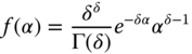
Hausman et al. (1984) also proposed a between and a random effects Poisson model, integrating out the relevant probabilities (9.33 et 9.34 respectively). A gamma distribution hypothesis is made for the individual effects, with the following density:

with

the gamma function. The expected value and the variance of ![]() are respectively:
are respectively:
If the model contains an intercept, the expected value is not identified and we can then suppose, without restriction, that it is equal to 1, which implies ![]() . We then obtain a gamma distribution with one parameter (denoted
. We then obtain a gamma distribution with one parameter (denoted ![]() ):
):
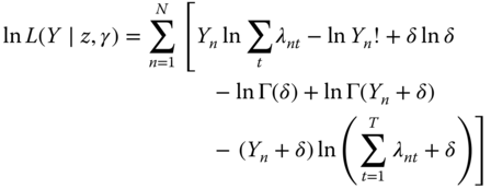
Integrating out the conditional probabilities (9.33 and 9.34), we obtain the unconditional probabilities for the between and the random effects models:

which leads to the following log‐likelihood functions:

9.3.3.2 The NegBin Model
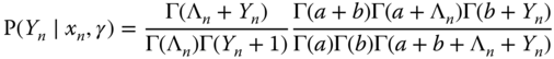
In addition to the Poisson model, Hausman et al. (1984) also proposed between and random effects NegBin models. We just present below without demonstration the joint probability for individual ![]() .
.

9.4 More Empirical Examples
Charness and Villeval (2009) investigate the difference in behavior between senior and junior workers in terms of risk aversion, competition, and cooperation. They conduct an experiment during which every participant can invest his or her initial endowment in a public good game, which is the explanatory variable of their econometric analysis. This variable is left‐ (null contribution) and right‐ (contribution of the full endowment) censored. As the participants are observed during 16 periods, they use a random effects tobit model. The Seniors data set is available in package pder.
Michalopoulos and Papaioannou (2016) explore the consequences of ethnic partitioning, which is one aspect of the “scramble for Africa” during which European countries partitioned Africa without caring much about the boundaries of ethnic groups. Their pseudo‐panel consists of 825 ethnic groups belonging to 49 countries. The authors estimate a Negbin model, where the response is the number of conflicts in an ethnicity‐country homeland, the major covariate being a dummy for partitioned ethnic areas. They introduce country fixed effects and estimate a specification where the fixed effects are estimated and not wiped out using a sufficient statistic. Partitioned ethnicities experience an increase of 57% in political violence compared to other areas. The data are available in package pder as ScrambleAfrica.
Bardhan and Mookherjee (2010) analyze the political determinants of land reform in West Bengal, India. More specifically, they use yearly data on 89 villages for the 1978‐1998 period. The response is the percentage of land or of households affected by land reform; it is highly censored, as it is 0 for more than 80% of the sample. The main covariate is the presence of a left‐wing coalition at the head of the local government. The authors use the trimmed least absolute deviation estimator of Honoré (1992) and don't find any significant effect of the left‐wing government variable on the strength of land reform. The LandReform data are available in package pder
Brandts and Cooper (2006) analyze how financial incentives can be used to overcome a history of coordination failure. For this purpose, they conduce an experiment where “firms,” composed of four “employees” have an output that is related to the lowest level of effort implemented by the employees. The individual or the lowest firm level effort is the response and, as the same employees/firms are observed during 30 different rounds, panel data techniques are used. The level of effort being ordinal, the authors use ordered probit models, with firm random effects and nested random effects respectively when the analysis is at the firm or at the employee level. Their dataset is available in the pder package as CoordFailure.
Farber et al. (2016) conducted an audit study to analyze the determinants of callbacks to job applications. They sent four fake resumes for 1,118 job openings and the response is a dummy indicating a callback, the covariates being the unemployment spell duration, the age, and the fact that the worker has held a low level interim job. They estimate a random effects and a conditional logit model with job opening effects. The Callbacks data are to be found in the pder package.
Bazzi (2017) investigates the influence of income on migration. At the household and at the village level, the response being in the first case a dummy that indicates whether a person in the household migrated during the given year and in the second case the percentage of the population of the village that has migrated. The main covariates are rainfall, rice price shock, and wealth at the household level and at the village level, indicators of the shape of wealth distribution. The author uses a conditional logit at the household level and the two‐sided trimmed least absolute deviations estimator (see Alan et al., 2013) at the village level. The IncomeMigrationV (village level) and IncomeMigrationH (household level) datasets are also included in the pder package.
Vella and Verbeek (1998) estimate the union premium for young men. In a first step, they estimate a dynamic random effect probit model for union membership. The UnionWage dataset is available in the pglm package.
Hausman et al. (1986) and Cincer (1997) study the dynamic relationship between patents and R&D using yearly panels of firms. They fit different count data models, including conditional Poisson and Negbin models. The data sets they used are available as PatentsRDUS and PatentsRD in the pglm packages.