
Chapter 5
Robust Inference and Estimation for Non‐spherical Errors
5.1 Robust Inference
In this chapter we focus on relaxing the hypothesis of independence and homoscedasticity of the remainder errors. Independent and identically distributed (i.i.d.) errors can seldom be taken for granted in the mostly non‐experimental contexts of econometrics. In the so‐called robust approach to model diagnostics, one relaxes the hypothesis of homoscedastic and independent errors from the beginning, and consequently uses an appropriate estimator for the parameters' covariance matrix, instead of testing for departures from sphericity after estimation, as is customary in the classical approach.
In panel data, error correlation often descends from clustering issues: the group (firm, individual, country) and the time dimension define natural clusters; observations sharing a common individual unit, or time period, are likely to share common characters, violating the independence assumption and potentially biasing inference. In particular, variance estimates derived under the random sampling assumption are typically biased downward, possibly leading to false significance of model parameters. Although clustering can often be an issue in cross‐sectional data too, especially when employing data at different levels of aggregation (Moulton, 1986, 1990), it is such an obvious feature in panels that a number of robust covariance estimators have been devised for the most common situations: within‐individual and/or ‐time period correlation, the former of either time‐constant or time‐decaying type, and cross correlation between different individuals over time.
Next to the panel‐specific implementation of the well‐known heteroscedasticity‐consistent covariance, there are a number of other robust covariance estimators specifically devised for panel data. We will now review the general idea of sandwich estimation, its application in a panel setting, and lastly the best known covariance estimators for the most common cases of nonsphericity in the errors and their implementations in plm.
5.1.1 Robust Covariance Estimators
Consider a linear model ![]() and the OLS estimator
and the OLS estimator ![]() . If the error terms
. If the error terms ![]() are independent and identically distributed, then the estimated covariance matrix of estimators takes the familiar textbook form:
are independent and identically distributed, then the estimated covariance matrix of estimators takes the familiar textbook form: ![]() , where
, where ![]() is an estimate of the error variance. This is the classical case, also known as spherical errors, and the relative formulation of
is an estimate of the error variance. This is the classical case, also known as spherical errors, and the relative formulation of ![]() is often referred to as “OLS covariance”.
is often referred to as “OLS covariance”.
Let us consider robust estimation in the context of the simple linear model outlined above. The problem at hand is to estimate the covariance matrix of the OLS estimator relaxing the assumptions of serial correlation and/or homoscedasticity without imposing any particular structure to the errors' variance or interdependence. The OLS parameters' covariance matrix with a general error covariance ![]() is:
is:
According to the seminal work of White (1980), in order to consistently estimate ![]() , it is not necessary to estimate all the
, it is not necessary to estimate all the ![]() unknown elements in the
unknown elements in the ![]() matrix but only the
matrix but only the ![]() ones in
ones in

which may be called the meat of the sandwich, the two ![]() being the bread. All that is required are pointwise consistent estimates of the errors, which is satisfied by consistency of the estimator for
being the bread. All that is required are pointwise consistent estimates of the errors, which is satisfied by consistency of the estimator for ![]() (see Greene, 2003). In the heteroscedasticity case, correlation between different observations is ruled out, and the meat reduces to
(see Greene, 2003). In the heteroscedasticity case, correlation between different observations is ruled out, and the meat reduces to
where the ![]() unknown
unknown ![]() s can be substituted by
s can be substituted by ![]() (see White, 1980). In the serial correlation case, the natural estimation counterpart would be
(see White, 1980). In the serial correlation case, the natural estimation counterpart would be ![]() but this structure proves too general to achieve convergence. Newey and West (1987) devise a heteroscedasticity and‐autocorrelation consistent estimator that works based on the assumption of correlation dying out as the distance between observations increases. The Newey‐West HAC estimator for the meat takes that of White and adds a sum of covariances between the different residuals, smoothed out by a kernel function giving weights decreasing with distance:
but this structure proves too general to achieve convergence. Newey and West (1987) devise a heteroscedasticity and‐autocorrelation consistent estimator that works based on the assumption of correlation dying out as the distance between observations increases. The Newey‐West HAC estimator for the meat takes that of White and adds a sum of covariances between the different residuals, smoothed out by a kernel function giving weights decreasing with distance:
with ![]() the weight from the kernel smoother. For the latter, Newey and West (1987) chose the well‐known Bartlett kernel function:
the weight from the kernel smoother. For the latter, Newey and West (1987) chose the well‐known Bartlett kernel function: ![]() . The lag
. The lag ![]() is usually truncated well below sample size: one popular rule of thumb is
is usually truncated well below sample size: one popular rule of thumb is ![]() (see Greene, 2003; Driscoll and Kraay, 1998).
(see Greene, 2003; Driscoll and Kraay, 1998).
In the following we will consider the extensions of this framework for a panel data setting where, thanks to added dimensionality, various combinations of the two above structures will turn out to be able to accommodate very general types of dependence.
5.1.1.1 Cluster‐robust Estimation in a Panel Setting
Clustering estimators extend the sandwich principle to panel data. Besides heteroscedasticity, the added dimensionality allows to obtain robustness against totally unrestricted time‐wise or cross‐sectional correlation, provided this is along the “smaller” dimension. In the case of “large‐![]() ” (wide) panels, the big cross‐sectional dimension allows robustness against serial correlation (Arellano, 1987); in “large‐
” (wide) panels, the big cross‐sectional dimension allows robustness against serial correlation (Arellano, 1987); in “large‐![]() ” (long) panels, on the converse, robustness to cross‐sectional correlation can be attained drawing on the large number of time periods observed. As a general rule, the estimator is asymptotic in the number of clusters.
” (long) panels, on the converse, robustness to cross‐sectional correlation can be attained drawing on the large number of time periods observed. As a general rule, the estimator is asymptotic in the number of clusters.
Imposing cross‐sectional (serial) independence in fact restricts all covariances between observations belonging to different individuals (time periods) to zero, yielding an error covariance matrix that is block‐diagonal, with blocks ![]() of the form:
of the form:
and the consistency relies on the cross‐sectional dimension being “large enough” with respect to the number of free covariance parameters in the diagonal blocks. The other case is symmetric.
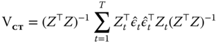
White's heteroscedasticity‐consistent covariance matrix has been extended to clustered data by Liang and Zeger (1986) and to econometric panel data by Arellano (1987). Observations can be clustered by the individual index, which is the most popular use of this estimator and is appropriate in large, short panels because it is based on ![]() ‐asymptotics, or by the time index, which is based on
‐asymptotics, or by the time index, which is based on ![]() ‐asymptotics and therefore appropriate for long panels. In the first case, the covariance estimator is robust against cross‐sectional heteroscedasticity and also against serial correlation of arbitrary form; in the second case, symmetrically, against time‐wise heteroscedasticity and cross‐sectional correlation. Arellano's original estimator, an instance of the first case, has the form:
‐asymptotics and therefore appropriate for long panels. In the first case, the covariance estimator is robust against cross‐sectional heteroscedasticity and also against serial correlation of arbitrary form; in the second case, symmetrically, against time‐wise heteroscedasticity and cross‐sectional correlation. Arellano's original estimator, an instance of the first case, has the form:
It is of course still feasible to rule out serial correlation and compute an estimator that is robust to heteroscedasticity only, based on the following error structure:
in which case the original White estimator applies:
The case of clustering by time period is symmetric to that along the other dimension: data are assumed to be serially independent and allowed to have arbitrary heteroscedasticity and an unrestricted cross‐sectional dependence structure.
Clustering in Non‐Panels
Clustering can occur in non‐panel settings too. Whenever a grouping index of some sort is provided and there is reason to believe that errors are dependent within groups defined by that index, the clustered standard errors can be employed to account for heteroscedasticity across groups and for within group correlation of any kind, not limited to proper serial correlation in time. One example is when a regression is augmented with variables at a higher level of aggregation.
The seminal example is in Moulton (1986, 1990): if some regressors are observed at group level, as is the case, e.g., when adding local GDP to individual data drawn from different geographical units, then standard errors have to be adjusted for intra‐group correlation.
Froot (1989), in the context of financial data, discusses sampling firms from different industries, assumed mutually independent. In his application, clustering is employed to account for within‐industry dependence, while it would be meaningless across the “other” dimension.
Any dataset mixing different levels of detail is prone to this issue. In such cases, panel data methods can seamlessly be employed on cross‐sectional datasets by specifying the relevant grouping variable as the first element of the index. The second one will obviously be left blank as there would be no meaningful second dimension.
5.1.1.2 Double Clustering
Double clustering methods have originated in the financial literature (Petersen, 2009; Cameron et al., 2011; Thompson, 2011) and are motivated by the need to account for persistent shocks (another name for individual, time‐invariant error components) and at the same time for cross‐sectional or spatial correlation. The former feature, persistent shocks, is usually dealt with in the econometric literature by parametric estimation of random effects models; the latter through spatial panels, where again it is estimated parametrically imposing a structure to the dependence, or common factor models. As Cameron et al. (2011) observe, though, double clustering, as all robustified inference of this kind, relies on much weaker assumptions as regards the data‐generating process than parametric modeling of dependence does. In fact, this estimator combining both individual and time clustering relies on a combination of the asymptotics of each: the minimum number of clusters along the two dimensions must go to infinity (which will be especially appropriate for data‐rich financial applications, less so in the smaller samples that are frequently encountered in economics). Apart from this, any dependence structure is allowed within each group or within each time period, while cross‐serial correlations between observations belonging to different groups and time periods are ruled out.
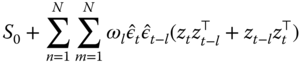
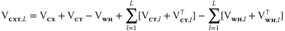
Cameron et al. (2011) have shown how the double‐clustered estimator is simply calculated by summing up the group‐clustering and the time‐clustering ones, then subtracting the standard White estimator in order to avoid double counting the error variances along the diagonal:
In order to control for the effect of common shocks, Thompson (2011) proposes to add to the sum of covariances one more term, related to the covariances between observations from any group at different points in time. Given a maximum lag ![]() , this will be the sum over
, this will be the sum over ![]() of the following generic term:
of the following generic term:
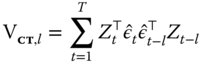
representing the covariance between pairs of observations from any group distanced ![]() periods in time. As the correlation between observations belonging to the same group at different points in time has already been captured by the group‐clustering term, to avoid double counting one must subtract the within‐groups part:
periods in time. As the correlation between observations belonging to the same group at different points in time has already been captured by the group‐clustering term, to avoid double counting one must subtract the within‐groups part:

for each ![]() . The resulting estimator
. The resulting estimator
is robust to cross‐sectional and time‐wise correlation inside, respectively, time periods and groups and to the cross‐serial correlation between observations belonging to different groups, up to the ![]() ‐th lag.
‐th lag.
5.1.1.3 Panel Newey‐west and SCC
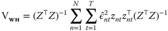
As mentioned above, in a time series context Newey and West (1987) have proposed an estimator that is robust to serial correlation as well as to heteroscedasticity. This estimator, based on the hypothesis of the serial correlation dying out “quickly enough,” takes into account the covariance between units by weighting it through a kernel‐smoothing function giving less weight as they get more distant and adding it to the standard White estimator.
A panel version of the original Newey‐West estimator can be obtained as:
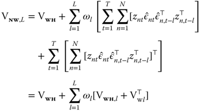
As can readily be seen, the Newey‐West non‐parametric estimator closely resembles the double clustering plus lags, the difference being that instead of adding a (possibly truncated) sum of unweighted lag terms, the latter downweighs the correlation between “distant” terms through a kernel‐smoothing function.
Driscoll and Kraay (1998) have adapted the Newey‐West estimator to a panel time series context where not only serial correlation between residuals from the same individual in different time periods is taken into account but also cross‐serial correlation between different individuals in different times and, within the same period, cross‐sectional correlation (see also Arellano, 2003).
The Driscoll and Kraay estimator, labeled SCC (as in “spatial correlation consistent”), is defined as the time‐clustering version of Arellano plus a sum of lagged covariance terms, weighted by a distance‐decreasing kernel function ![]() :
:
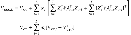
The “SCC” covariance estimator requires the data to be a mixing sequence, i.e., roughly speaking, to have serial and cross‐serial dependence dying out quickly enough with the ![]() dimension, which is therefore supposed to be fairly large: Driscoll and Kraay (1998), based on Monte Carlo simulation, put the practical minimum at
dimension, which is therefore supposed to be fairly large: Driscoll and Kraay (1998), based on Monte Carlo simulation, put the practical minimum at ![]() ; the
; the ![]() dimension is irrelevant in this respect and is allowed to grow at any rate relative to
dimension is irrelevant in this respect and is allowed to grow at any rate relative to ![]() .
.
As is apparent from Equation 5.1.1.3, if the maximum lag order is set to 0 (no serial or cross‐serial dependence is allowed) the SCC estimator becomes the cross‐section version (time‐clustering) of the Arellano estimator ![]() . On the other hand, if the cross‐serial terms are all unweighted (i.e., if
. On the other hand, if the cross‐serial terms are all unweighted (i.e., if ![]() ), then
), then ![]() .
.
A Comprehensive Definition
Let us now look systematically at the similarities between the above formulas, embedding them into an encompassing one (see Millo, 2017b). A comprehensive formulation can be written in terms of White's heteroscedasticity‐consistent covariance matrix ![]() , the group‐clustering and time‐clustering ones
, the group‐clustering and time‐clustering ones ![]() and
and ![]() , and an appropriate kernel‐weighted sum of their lags:
, and an appropriate kernel‐weighted sum of their lags:

The different estimators are in turn particularizations of the above and can be expressed in terms of the same basic common components, as shown in Table 5.1. A function vcovG making either ![]() ,
, ![]() , or
, or ![]() is provided at user level, mainly for educational purposes, and is used internally to construct all other estimators.1
is provided at user level, mainly for educational purposes, and is used internally to construct all other estimators.1
Table 5.1 Covariance structures as combinations of the basic building blocks.
| double‐clustering | |
| time‐clustering + shocks | |
| panel Newey‐West | |
| Driscoll and Kraay's SCC | |
| double‐clustering + shocks | |
Higher‐level functions are provided to produce the double‐clustering and kernel‐smoothing estimators by (possibly weighted) sums of the former terms. The general tool in this respect, in turn based on vcovG, is vcovSCC, which computes weighted sums of ![]() according to a weighting function that is by default the Bartlett kernel. The default values will yield the Driscoll and Kraay estimator,
according to a weighting function that is by default the Bartlett kernel. The default values will yield the Driscoll and Kraay estimator, ![]() . As the SCC estimator differs from the (one‐way) time‐shocks‐robust version of the double‐clustering a la Cameron et al. (2011) only by the distance‐decaying weighting of the covariances between different periods so that
. As the SCC estimator differs from the (one‐way) time‐shocks‐robust version of the double‐clustering a la Cameron et al. (2011) only by the distance‐decaying weighting of the covariances between different periods so that ![]() , no weighting (equivalent to passing the constant 1 as the weighting function:
, no weighting (equivalent to passing the constant 1 as the weighting function: wj=1) will produce the building blocks for double clustering, according to formula 5.9.
Convenient wrappers are provided as the tool of choice for the end user: vcovNW computes the panel Newey‐West estimator ![]() ;
; vcovDC the double‐clustering one ![]() .
.
5.1.2 Generic Sandwich Estimators and Panel Models
plm provides a comprehensive set of modular tools: lower‐level components, conceptually corresponding to the statistical “objects” involved, (see Zeileis, 2006a,b), and a higher‐level set of “wrapper functions” corresponding to standard parameter covariance estimators as they would be used in statistical packages, which work by combining the same, few lower‐level components in multiple ways in the spirit of the Lego principle of Hothorn et al. (2006).
When estimating regression models, R creates a model object that, together with estimation results, carries on a wealth of useful information, including the original data. Robust testing in R is done retrieving the necessary elements from the model object, using them to calculate a robust covariance matrix for coefficient estimates and then feeding the latter to the actual test function, for example a t‐test for significance or a Wald restriction test. This approach to diagnostic testing is more flexible than with standard econometric software packages, where diagnostics usually come with standard output. In our case, for example, one can obtain different estimates of the standard errors under various kinds of dependence without re‐estimating the model and present them compactly.
Robust covariance estimators a la White or a la Newey and West for different kinds of regression models are available in package sandwich (Lumley and Zeileis, 2007) under form of appropriate methods for the generic functions vcovHC and vcovHAC (Zeileis, 2004, 2006a). These are designed for data sampled along one dimension; therefore, they cannot generally be used for panel data, yet they provide a uniform and flexible software approach, which has become standard in the R environment. The corresponding plm methods described in this chapter have therefore been designed to be sintactically compliant with them.
For example, a vcovHC.plm method for the generic vcovHC is available, allowing to apply sandwich estimators to panel models in a way that is natural for users of the sandwich package. In fact, despite the different structure “under the hood,” the user will, e.g., specify a robust covariance for the diagnostics table of a panel model the same way she would for a linear or a generalized linear model, the object‐orientation features of R taking care that the right statistical procedure be applied to the model object at hand. What will change, though, are the defaults: the vcovHC.lm method defaults to the original White estimator, while vcovHC.plm to clustering by groups, both the most obvious choices for the object at hand.
Next to the HC estimator of White (1980), all variants of the panel‐specific estimators used in applied practice (Arellano, 1987; Newey and West, 1987; Driscoll and Kraay, 1998; Cameron et al., 2011) are provided; all can be applied to objects representing panel models of different kinds: FE, RE, FD, and, obviously, pooled OLS. The estimate of the parameters' covariance thus obtained can in turn be plugged into diagnostic testing functions, producing either significance tables or hypothesis tests. A function is a regular object type in R, hence compact comparisons of standard errors from different (statistical) methods can be produced by looping on covariance types, as shown in the examples.
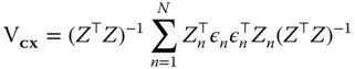
Application to Models on Transformed Data
The application of the above estimators to pooled data is always warranted, subject to the relevant assumptions mentioned before. In some, but not all cases, these can also be applied to random or fixed effects panel models, or models estimated on first‐differenced data. In all of these cases the estimator is computed as OLS on transformed (partially or totally demeaned, first differenced) data. In general, the same transformation used in estimation is employed. Sandwich estimators can then be computed by applying the usual formula to the transformed data and residuals: ![]() (see Arellano (1987) and Wooldridge (2002, Eq. 10.59) for the fixed effects case, Wooldridge (2002, Ch.10) in general).
(see Arellano (1987) and Wooldridge (2002, Eq. 10.59) for the fixed effects case, Wooldridge (2002, Ch.10) in general).
Under the fixed effects hypothesis, the OLS estimator is biased and FE is required for consistency of parameter estimates in the first place. Similarly, under the hypothesis of a unit root in the errors, first differencing the data is warranted in order to revert to a stationary error term. On the contrary, under the random effects hypothesis, OLS is still consistent, and asymptotically, using RE instead makes no difference. Yet for the sake of parameter covariance estimation, it may be advisable to eliminate time‐invariant heterogeneity first, by using one of the above.
One compelling reason for combining a demeaning or a differencing estimator with robust standard errors may be to get rid of persistent individual effects before applying a more parsimonious and efficient kernel‐based covariance estimator if cross‐serial correlation is suspected or if the sample is simply not big enough to allow double clustering. In fact, as Petersen (2009) shows, the Newey‐West‐ type estimators are biased if effects are persistent, because the kernel smoother unduly downweighs the covariance between faraway observations.
In the following we discuss when it is appropriate to apply clustering estimators to the residuals of demeaned or first‐differenced models.
Fixed Effects
The fixed effects estimator requires particular caution. In fact, under the hypothesis of spherical errors in the original model, the time‐demeaning of data induces a serial correlation ![]() in the demeaned residuals (see Wooldridge, 2002, p. 310).
in the demeaned residuals (see Wooldridge, 2002, p. 310).
The White‐Arellano estimator has originally been devised for this case. By way of symmetry, it can be used for time‐clustered data with time fixed effects. The combination of group clustering with time fixed effects and the reverse is inappropriate because of the serial (cross‐sectional) correlation induced by the time‐ (cross‐sectional‐) demeaning.
By analogy, the Newey‐West‐type estimators can be safely applied to models with individual fixed effects, while the time and two‐way cases require caution. The best policy in both cases, if the degrees of freedom allow, is perhaps to explicitly add dummy variables to account for the fixed effects along the “short” dimension.
Random Effects
In the random effects case, as Wooldridge (2002) notes, the quasi‐time demeaning procedure removes the random effects reducing the model on transformed data to a pooled regression, thus preserving the properties of the White‐type estimators. By extension of this line of reasoning, all above estimators are applicable to the demeaned data of a random effects model, provided the transformed errors meet the relevant assumptions.
First‐Differences
First‐differencing, like fixed effects estimation, removes time‐invariant effects. Roughly speaking, the choice between the two rests on the properties of the error term: if it is assumed to be well behaved in the original data, then FE is the most efficient estimator and is to be preferred; if on the contrary the original errors are believed to behave as a random walk, then first‐differencing the data will yield stationary and uncorrelated errors and is therefore advisable (see Wooldridge, 2002, p. 317). Given this, FD estimation is nothing else than OLS on differenced data, and the usual clustering formula applies (see Wooldridge, 2002, p. 318 and Chapter here). As in the RE case, the statistical properties of the different covariance estimators will depend on whether the transformed errors meet the relevant assumptions.
5.1.2.1 Panel Corrected Standard Errors
Unconditional covariance estimators are based on the assumption of no error correlation in time (cross‐section) and of an unrestricted but invariant correlation structure inside every cross section (time period). 3 They are popular in contexts characterized by relatively small samples, with prevalence of the time dimension. The most common use is on pooled time series, where the assumption of no serial correlation can be accommodated, for example, by adding lagged values of the dependent variable.
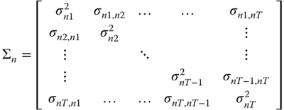
Beck and Katz (1995), in the context of political science models with moderate time and cross‐sectional dimensions, introduced the so‐called panel corrected standard errors (PCSE), which, in the original time‐clustering setting, are robust against cross‐sectional heteroscedasticity and correlation. The “PCSE” covariance is based on the hypothesis that the covariance matrix of the errors in every group be the same: ![]() , with
, with
so that ![]() can be estimated by:
can be estimated by:
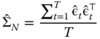
from which ![]() can be constructed and inserted in the usual “sandwich” formula.
can be constructed and inserted in the usual “sandwich” formula.
5.1.3 Robust Testing of Linear Hypotheses
The main use of robust covariance estimators is together with testing functions from the lmtest (Zeileis and Hothorn, 2002) and car (Fox and Weisberg, 2011) packages. We have seen the special case of testing single exclusion restrictions through coeftest: in order of increasing generality, joint restrictions can be tested through waldtest, while linearHypothesis from package car enables testing a general linear hypothesis on model parameters.
For some tests, e.g., for multiple model comparisons by waldtest, one should always provide a function.
5.1.3.1 An Application: Robust Hausman Testing
Beside the usual quadratic form, Hausman's specification test can be performed in an equivalent form based on testing a linear restriction in an auxiliary linear model. In particular, it can be computed through an artificial regression of the quasi‐demeaned response over the quasi‐demeaned regressors from the random effects augmented with the fully demeaned regressors from the within model:
The Hausman test is then the redundancy test on ![]() , i.e., the restriction test
, i.e., the restriction test ![]() . This artificial regression version of the test can easily be robustified (see Wooldridge, 2002) by using a robust covariance matrix.
. This artificial regression version of the test can easily be robustified (see Wooldridge, 2002) by using a robust covariance matrix.
5.2 Unrestricted Generalized Least Squares
If the data‐generating process is:
and ![]() has a general structure, ordinary least squares estimates for
has a general structure, ordinary least squares estimates for ![]() are inefficient, though consistent. By Aitken's theorem (see, e.g., Greene (2003), 10.5), generalized least squares (GLS) are the efficient estimator for the model parameters if
are inefficient, though consistent. By Aitken's theorem (see, e.g., Greene (2003), 10.5), generalized least squares (GLS) are the efficient estimator for the model parameters if ![]() is known. The estimator is then
is known. The estimator is then
Various feasible GLS procedures exist drawing on consistent estimators of ![]() , which are then plugged into the GLS estimator. The key to obtaining a consistent estimate of
, which are then plugged into the GLS estimator. The key to obtaining a consistent estimate of ![]() is, in general, to specify enough structure to faithfully represent its characteristics while keeping the number of parameters to be estimated at a manageable level.
is, in general, to specify enough structure to faithfully represent its characteristics while keeping the number of parameters to be estimated at a manageable level.
In the standard one‐way error components model, as already seen, the disturbance term may be written as ![]() where
where ![]() denotes the (time‐invariant) individual‐specific effect and
denotes the (time‐invariant) individual‐specific effect and ![]() the idiosyncratic error. Observations regarding the same individual
the idiosyncratic error. Observations regarding the same individual ![]() share the same
share the same ![]() effect, thus the relative errors are autocorrelated. The random effects structure is a very parsimonious way to account for individual heterogeneity, which can be extended in various dimensions, e.g., by specifying an autoregressive process in space and/or time for the idiosyncratic component
effect, thus the relative errors are autocorrelated. The random effects structure is a very parsimonious way to account for individual heterogeneity, which can be extended in various dimensions, e.g., by specifying an autoregressive process in space and/or time for the idiosyncratic component ![]() .
.
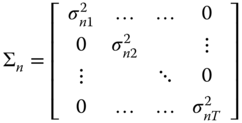
Under the random effects specification, the variance‐covariance matrix of the errors ![]() is block‐diagonal with
is block‐diagonal with ![]() where
where
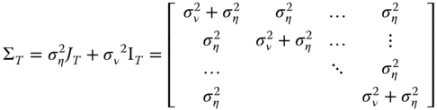
The above is the standard specification of random effects panels, described in the previous chapters. It parsimoniously describes the error covariance by means of just two parameters and is, therefore, of very general applicability as far as sample sizes are concerned. In panels with one dimension much larger than the other (typically, large and short panels) a less restrictive approach is possible, termed general GLS (Wooldridge, 2002, 10.4.3), which allows for arbitrary within‐individual heteroscedasticity and serial correlation of errors, i.e., inside the ![]() covariance submatrices, provided that these remain the same for every individual.
covariance submatrices, provided that these remain the same for every individual.
5.2.1 General Feasible Generalized Least Squares
If one assumes ![]() but leaves the structure of
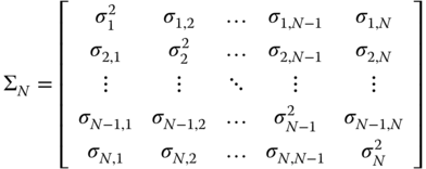
but leaves the structure of ![]() completely free except for the obvious requisites of being symmetric and positive definite:
completely free except for the obvious requisites of being symmetric and positive definite:
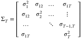
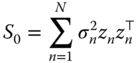
individual errors can evolve through time with an unlimited amount of heteroscedasticity and autocorrelation, but they are assumed to be uncorrelated between them in the cross section, and this structure is assumed constant over the different individuals. By this assumption, the components ![]() of
of ![]() can be estimated drawing on the cross‐sectional dimension, using the average over individuals of the outer products of the residuals from a consistent estimator:
can be estimated drawing on the cross‐sectional dimension, using the average over individuals of the outer products of the residuals from a consistent estimator:
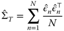
where ![]() is the subvector of OLS residuals for individual
is the subvector of OLS residuals for individual ![]() .
.
This estimator is called general feasible GLS, or GGLS and is also sometimes referred to as the Parks (1967) estimator and is, as observed by Driscoll and Kraay (1998), a variant of the SUR estimator by Zellner (1962). Greene (2003) presents the same estimator in the context of pooled time series, with fixed ![]() and “large”
and “large” ![]() .
.
Leaving the intra‐group error covariance parameters completely free to vary is an attractive strategy, provided that ![]() because the number of variance parameters to be estimated with
because the number of variance parameters to be estimated with ![]() data points is
data points is ![]() (Wooldridge, 2002). This is a typical situation in micro‐panels such as, e.g., household income surveys, where
(Wooldridge, 2002). This is a typical situation in micro‐panels such as, e.g., household income surveys, where ![]() is in the thousands but
is in the thousands but ![]() is typically quite short so that even if estimating an unrestricted covariance, many degrees of freedom are still available.
is typically quite short so that even if estimating an unrestricted covariance, many degrees of freedom are still available.
The original applications have instead been in the field of pooled time series, aimed at accounting for cross‐sectional correlation and heteroscedasticity. In this context, Driscoll and Kraay (1998) observe how the lack of degrees of freedom in estimating the error covariance leads to near‐singular estimates and hence to downward‐biased standard errors, thus overestimating parameter significance. Beck and Katz (1995) also discuss some severe biases of this estimator in small samples. Both start from a pooled time series, ![]() ‐asymptotic approach, and both are interested in robustness over the cross‐sectional dimension. In this light, most of the criticism this estimator has been subject to depends on the peculiar field of application, especially in Beck and Katz (1995) and references therein (Alvarez et al., 1991) where it is applied to political science data with very modest sample sizes; but recent simulations by Chen et al. (2009) show that even in such situations FGLS can be more efficient than the proposed alternatives (OLS with PCSE standard errors).
‐asymptotic approach, and both are interested in robustness over the cross‐sectional dimension. In this light, most of the criticism this estimator has been subject to depends on the peculiar field of application, especially in Beck and Katz (1995) and references therein (Alvarez et al., 1991) where it is applied to political science data with very modest sample sizes; but recent simulations by Chen et al. (2009) show that even in such situations FGLS can be more efficient than the proposed alternatives (OLS with PCSE standard errors).
The GGLS principle can be applied to various situations, consistent with different views on heterogeneity (random vs fixed effects hypothesis) or stationarity (e.g., to a model in first differences). That translates into either applying the unrestricted GLS estimator directly to the observed data or to a transformation thereof.
This framework allows the error covariance structure inside every group (if effect is set to 'individual') of observations to be fully unrestricted and is therefore robust against any type of intra‐group heteroscedasticity and serial correlation. This structure, by converse, is assumed identical across groups and thus general FGLS is inefficient under group‐wise heteroscedasticity. Cross‐sectional correlation is excluded a priori.
In a pooled time series context (effect is set to 'time'), symmetrically, this estimator is able to account for arbitrary cross‐sectional correlation, provided that the latter is time invariant (see Greene, 2003, 13.9.1–2, p. 321–322). In this case, serial correlation has to be assumed away and the estimator is consistent with respect to the time dimension, keeping ![]() fixed.
fixed.
5.2.1.1 Pooled GGLS
Under the specification described at the beginning of this section, residuals can be consistently estimated by OLS and then used to estimate ![]() as above. Using
as above. Using ![]() , the FGLS estimator is:
, the FGLS estimator is:
The estimated individual submatrix ![]() will give an assessment of the structure, if any, of the errors' covariance, which may guide towards more parsimonious specifications like the RE one (if all diagonal and, respectively, all off‐diagonal elements are of similar magnitude) or possibly an AR(1) specification, if covariances between pairs of off‐diagonal elements become smaller with distance.
will give an assessment of the structure, if any, of the errors' covariance, which may guide towards more parsimonious specifications like the RE one (if all diagonal and, respectively, all off‐diagonal elements are of similar magnitude) or possibly an AR(1) specification, if covariances between pairs of off‐diagonal elements become smaller with distance.
In this small‐![]() , large‐
, large‐![]() context, one will often want to include time fixed effects to mitigate cross‐sectional correlation, which is assumed out of the residuals.
context, one will often want to include time fixed effects to mitigate cross‐sectional correlation, which is assumed out of the residuals.
The function pggls estimates general FGLS models, either with or without fixed effects, or on first‐differenced data. In the following we illustrate it on the EmplUK data.
5.2.1.2 Fixed Effects GLS
If individual heterogeneity is present but we do not trust the random effects assumption, and moreover the remainder errors are expected to show heteroscedasticity and serial correlation, the FE estimator can be employed together with a robust covariance matrix; but if the cross‐sectional dimension is sufficient and the assumption of constant covariance matrix across individuals is realistic, then applying the GGLS method to time‐demeaned data can provide a more efficient alternative, called the fixed effects GLS (![]() ) estimator (Wooldridge, 2002, 10.5.5).5
) estimator (Wooldridge, 2002, 10.5.5).5
The errors covariance submatrix for each individual is now:

where ![]() is the subvector of FE (within) residuals for individual
is the subvector of FE (within) residuals for individual ![]() . Using
. Using ![]() and the within transformed data, the
and the within transformed data, the ![]() estimator is:
estimator is:
This estimator, originally due to Kiefer (1980), takes care of both the serial correlation present in the original errors ![]() and, implicitly, of that induced by the demeaning. For this reason, being a combination of both, the estimated
and, implicitly, of that induced by the demeaning. For this reason, being a combination of both, the estimated ![]() does not give a direct assessment of the original error structure anymore.
does not give a direct assessment of the original error structure anymore.
5.2.1.3 First Difference GLS
Analogously, the GGLS principle can be applied to data in first differences, in the very same way as for ![]() , giving rise to the first difference GLS (
, giving rise to the first difference GLS (![]() ) estimator (Wooldridge, 2002, p. 320).
) estimator (Wooldridge, 2002, p. 320).
In this case, the errors covariance submatrix for an individual is:

where ![]() is the subvector of FD residuals for individual
is the subvector of FD residuals for individual ![]() . Using
. Using ![]() and the differenced data, the
and the differenced data, the ![]() estimator is:
estimator is:
First differencing eliminates time‐invariant unobserved heterogeneity, as does the within transformation; one difference is that now one time period is lost for each individual. FD has to be preferred to FE when the original data are likely to be nonstationary, because then the FD‐transformed residuals will be. Again, elements of ![]() do not directly represent the correlation structure of residuals because of the induced correlation from first differencing.
do not directly represent the correlation structure of residuals because of the induced correlation from first differencing.
To choose which method to use, one can look at the stationarity properties of the residuals. If the residuals of the ![]() estimator are not stationary, then
estimator are not stationary, then ![]() will be a more appropriate estimator.
will be a more appropriate estimator.