
Chapter 4
Tests on Error Component Models
The double dimensionality of panel data allows for much richer specifications than simple cross sections or time series. This is both a blessing and a curse, given how much more complicated the specification may become. In fact, all possible features from either cross sections or time series, like distance‐decaying correlation in – respectively – space or time, can coexist with individual (time), time‐(individual‐) invariant heterogeneity. Moreover, diagnostic tests will usually have a hard time distinguishing between different forms of persistence along the same dimension unless explicitly designed to take the “other” effect into account.
The specification problem of panel models is typically associated with the presence or absence of individual effects, i.e., with the need to account for unobserved heterogeneity. Given that in the vast majority of cases it will be inappropriate to rule out individual heterogeneity altogether, the related issue emerges of whether it is safe to assume that the latter is uncorrelated with the explanatory variables (and therefore to proceed in a random effects framework) or rather to proceed estimating out (transforming out) the individual effects in a fixed effects fashion. Hence, tests for individual effects under either of the two approaches and Hausman‐type tests for determining which one is appropriate are among the most popular diagnostic procedures in this field.
Next to the fundamental specification issues with individual effects , the remainder errors can in turn be correlated: either in time, in which case it will be crucial to distinguish time‐decaying persistence of idiosyncratic shocks from the time‐invariant persistence deriving from the presence of an individual effect; or in space, and then the issue becomes whether correlation simply descends from participating in the same cross section or, provided the data are referenced in some space (e.g., in geography), whether nearby observations are more correlated than distant ones.
For these reasons, a rich toolbox of diagnostic and specification testing procedures has been developed, which will be the subject of this chapter, presented roughly in the order given above up to the issue of cross‐sectional correlation. On the converse, spatial correlation proper will be the subject of a separate chapter.
4.1 Tests on Individual and/or Time Effects
In order to test whether either individual or time effects are present, two approaches are possible:
- the first is to start from estimating said effects out (within model) and then perform a zero restriction test,
- the second is to start from the OLS model and to infer about the presence of the effects drawing on the OLS residuals.
4.1.1 F Tests
The sum of squared residuals and the degrees of freedom for the within model are: ![]() and
and ![]() . Let the null hypothesis be the absence of individual effects so that the restricted model is pooled OLS where the sum of squared residuals and the degrees of freedom are, respectively,
. Let the null hypothesis be the absence of individual effects so that the restricted model is pooled OLS where the sum of squared residuals and the degrees of freedom are, respectively, ![]() and
and ![]() . Under
. Under ![]() , the test statistic:
, the test statistic:

follows a Fisher‐Snedecor F with ![]() and
and ![]() degrees of freedom.
degrees of freedom.
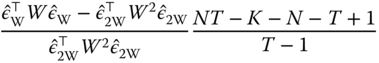
The test of the null hypothesis of no individual and time effects is obtained by using the two‐ways within model and the pooling model:

Finally, the test of the null hypothesis of, say, no time effects, but in the presence of individual effects is:
4.1.2 Breusch‐Pagan Tests
The Breusch and Pagan (1980) test is a Lagrange multipliers test based on the OLS residuals. It is based on the score vector ![]() , i.e., the vector of partial derivatives of the log‐likelihood function from the restricted model. The variance of the score vector is the information matrix:
, i.e., the vector of partial derivatives of the log‐likelihood function from the restricted model. The variance of the score vector is the information matrix:

We estimate a restricted model characterized by a parameter vector ![]() ; under
; under ![]() , we have:
, we have:
or, denoting by ![]() and
and ![]() the score and its estimated variance in the restricted model:
the score and its estimated variance in the restricted model:
which is distributed as a ![]() where the degrees of freedom are equal to the number of restrictions. We'll first derive the test for the one‐way individual error component model, for which the log‐likelihood function is:
where the degrees of freedom are equal to the number of restrictions. We'll first derive the test for the one‐way individual error component model, for which the log‐likelihood function is:

The gradient is then:

To derive the variance, we start by calculating the matrix of second derivatives ![]() :
:

To compute the expectation of this matrix, we note that ![]() and
and ![]() :
:

To compute the test statistic, we impose the null hypothesis: ![]() (absence of individual effects). In this case, the estimator for the parameters is OLS and that of
(absence of individual effects). In this case, the estimator for the parameters is OLS and that of ![]() is
is ![]() . The score and its estimated variance are then:
. The score and its estimated variance are then:

whose inverse is:

Finally, the test statistic is:
Or, replacing ![]() by
by ![]() :
:
which is asymptotically distributed as a ![]() with 1 degree of freedom.
with 1 degree of freedom.
The test of the time effect is likewise computed:

The Breusch‐Pagan test extends easily to the two‐ways error component model, as the statistic can be written as the sum of the two previous statistics:

and follows a ![]() with two degrees of freedom under the null hypothesis of no individual and time effects.
with two degrees of freedom under the null hypothesis of no individual and time effects.
For unbalanced panels, the relevant statistics are:1

These statistics present two problems. The first one is that the alternative hypothesis is that the effects' variance is non‐zero, i.e., strictly positive or negative; when a variance must be non‐negative. For the one‐way error component model, Honda (1985) and King and Wu (1997) proposed a one‐sided test based on the square root of the above statistic, which is then normally distributed. The Honda statistic is then ![]() and its 5% critical value is 1.64 (and likewise for the test of no time effects). For the two‐ways error components model, Honda (1985) proposed to use
and its 5% critical value is 1.64 (and likewise for the test of no time effects). For the two‐ways error components model, Honda (1985) proposed to use ![]() as Baltagi et al. (1992) and King and Wu (1997) use:
as Baltagi et al. (1992) and King and Wu (1997) use:

The second problem is due to the fact that ![]() or
or ![]() may be lower than 1. In this case, Baltagi et al. (1992), following Gourieroux et al. (1982), proposed to replace the statistic by 0. The modified statistic is then defined by:
may be lower than 1. In this case, Baltagi et al. (1992), following Gourieroux et al. (1982), proposed to replace the statistic by 0. The modified statistic is then defined by:

which follows a mixed ![]() distribution:
distribution: ![]()
4.2 Tests for Correlated Effects
We have seen that if the model errors are not correlated with the explanatory variables, then both estimators, fixed as well as random effects, are consistent. To compare them, we keep assuming that the idiosyncratic component of the error term (![]() ) is uncorrelated to the regressors. Two situations are then possible:
) is uncorrelated to the regressors. Two situations are then possible:
 : the individual effects are not correlated with the explanatory variables; in this case, both estimators are consistent, but the random effects estimator is more efficient than the fixed effects.
 : the individual effects are correlated with the explanatory variables; in this case, the fixed effects estimator, which estimates out the individual effects, is consistent. On the contrary, the random effects estimator is inconsistent because one component of the composite error, the individual effect, is correlated with the explanatory variables.
4.2.1 The Mundlak Approach
In order to clarify the relationship between the two estimators, Mundlak (1978) considered the following model:
with
The individual effects are therefore correlated with the explanatory variables, being they equal to the sum of a linear combination of the individual means of said variables and of an error term ![]() . The model to be estimated is then written, in matrix form, as:
. The model to be estimated is then written, in matrix form, as:
The error term ![]() has the usual properties of the error components model, i.e., zero mean and a variance equal to:
has the usual properties of the error components model, i.e., zero mean and a variance equal to:
The GLS model is estimated by applying OLS on the data transformed pre‐multiplying each variable by ![]() , with
, with ![]() .
.
We then have ![]() ,
, ![]() and
and ![]() . The GLS estimator is then written as:
. The GLS estimator is then written as:

Using the formula of the inverse of a partitioned matrix (see equation 2.19), we get:
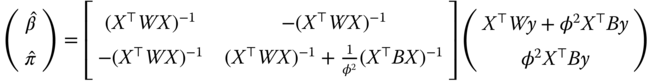
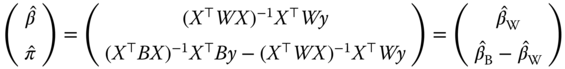
and:

The fundamental result of Mundlak (1978) is therefore that, if one correctly accounts for the correlation between the error terms and the explanatory variables, the GLS estimator is the within estimator.
4.2.2 Hausman Test
This results also suggests a way to test for the presence of correlation; in fact, testing for no correlation corresponds to testing for: ![]() . Under
. Under ![]() , we have:
, we have:
which is distributed as a ![]() with
with ![]() degrees of freedom. Well, we have
degrees of freedom. Well, we have ![]() and
and ![]() .
.
This test statistic is one version of the test proposed by Hausman (1978). The general principle consists in comparing two models ![]() and
and ![]() where:
where:
- under
 :
:  and
and  are both consistent, but
  is more efficient than
  ,
, - under
 : only
  is consistent.
The idea of the test is that if ![]() is true, then the estimated coefficients from the two models shall not diverge; under the alternative, they will. The test is therefore based on
is true, then the estimated coefficients from the two models shall not diverge; under the alternative, they will. The test is therefore based on ![]() and Hausman showed that, under
and Hausman showed that, under ![]() , the variance of this difference is simply:
, the variance of this difference is simply: ![]() .
.
The most common version of this test is based on comparing the within and the GLS estimators. The difference between the two is: ![]() . Under the hypothesis of no correlation between errors and explanatory variables, we have
. Under the hypothesis of no correlation between errors and explanatory variables, we have ![]() . The variance of
. The variance of ![]() is:
is:
To determine these variances and covariances, we write the two estimators as functions of the errors: ![]() and
and ![]() . We then have:
. We then have: ![]() ,
, ![]() and
and ![]() . The variance of
. The variance of ![]() is then simply:
is then simply:
and the test statistic becomes:
which, under ![]() , is distributed as a
, is distributed as a ![]() with
with ![]() degrees of freedom.
degrees of freedom.
4.2.3 Chamberlain's Approach
Chamberlain (1982) proposed a more general model than that of Mundlak (1978). In his model, the individual effects are not assumed to be a linear function of the means of the explanatory variables anymore, but of their values over the whole time period.
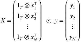
Denote ![]() the vector of length
the vector of length ![]() containing the values of the explanatory variables for the
containing the values of the explanatory variables for the ![]() ‐th individual, and
‐th individual, and ![]() the
the ![]() matrix containing the values of
matrix containing the values of ![]() explanatory variables for the
explanatory variables for the ![]() observation periods for the
observation periods for the ![]() ‐th individual.
‐th individual. ![]() is a vector of length
is a vector of length ![]() obtained by stacking the columns of
obtained by stacking the columns of ![]() . The model is then written as:
. The model is then written as:
with:
Substituting (4.2) in (4.1), we get:
The parameter matrix ![]() , of dimension
, of dimension ![]() , contains two types of parameters:
, contains two types of parameters:
- the vector of parameters
 , which measure the marginal effect of the explanatory variables on the response,
 - the vector of parameters
 , measuring the marginal effect of the explanatory variables in each period on the individual effect.
The ![]() vector is only marginally interesting per se, but its estimation allows to consistently estimate
vector is only marginally interesting per se, but its estimation allows to consistently estimate ![]() . If
. If ![]() and
and ![]() , the
, the ![]() matrix takes the form:
matrix takes the form:

We then have a system of ![]() equations containing the same explanatory variables
equations containing the same explanatory variables ![]() . In this case, the generalized least squares estimator is the SUR estimator. The explanatory variables being the same across equations, this can be obtained simply by estimating each individual equation separately by OLS. If the assumptions of the fixed effects model hold, then the estimation of each column of the
. In this case, the generalized least squares estimator is the SUR estimator. The explanatory variables being the same across equations, this can be obtained simply by estimating each individual equation separately by OLS. If the assumptions of the fixed effects model hold, then the estimation of each column of the ![]() matrix will yield just about equal coefficients, with the exception of those situated on the diagonal.
matrix will yield just about equal coefficients, with the exception of those situated on the diagonal.
4.2.3.1 Unconstrained Estimator
The coefficients of the ![]() row of
row of ![]() are then:
are then:

More generally, we can write the estimator of ![]() in two different ways. The first consists in defining:
in two different ways. The first consists in defining:
We have then:
In order to analyze the properties of this estimator, it is easier to consider the vector of coefficients ![]() obtained by stacking the rows of
obtained by stacking the rows of ![]() . Defining:
. Defining:
Denoting ![]() and substituting, in the last expression,
and substituting, in the last expression, ![]() by its expression in the “true” model:
by its expression in the “true” model:

The limiting distribution of ![]() is the same as that of:
is the same as that of:
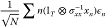
with ![]() because
because ![]() .
.
As ![]() , the central limit theorem implies that:
, the central limit theorem implies that:

If the error variance of ![]() is not correlated with
is not correlated with ![]() , this matrix simplifies to:
, this matrix simplifies to:
Finally, if the errors are homoscedastic, we get an even simpler expression:
with ![]() .
.
An estimator of ![]() can be obtained considering the sample equivalent. Denoting by
can be obtained considering the sample equivalent. Denoting by ![]() the estimation residuals, we get:
the estimation residuals, we get:

4.2.3.2 Constrained Estimator
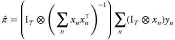
In a second time, Chamberlain (1982) utilizes the asymptotic least squares estimator in order to obtain an estimator of the structural coefficients of the model, denoted by ![]() . These are made of the
. These are made of the ![]() coefficients associated to the explanatory variables of equation 4.1) and of the
coefficients associated to the explanatory variables of equation 4.1) and of the ![]() coefficients from equation 4.2) concerning the individual effects. There are therefore
coefficients from equation 4.2) concerning the individual effects. There are therefore ![]() structural coefficients, while the number of coefficients in the matrix
structural coefficients, while the number of coefficients in the matrix ![]() is
is ![]() . The relation between the two coefficient vectors can be expressed as
. The relation between the two coefficient vectors can be expressed as ![]() ,
, ![]() being a matrix of dimensions
being a matrix of dimensions ![]() .
.
The restricted model is obtained employing the method of asymptotic least squares, consisting in minimizing a quadratic form in the deviations between ![]() and
and ![]() :
:
The first‐order conditions for a minimum can be written as:
which yields the following estimator:
This estimator is consistent regardless of the weighting matrix employed. Just as with the generalized method of moments, the estimator is efficient if ![]() is the covariance matrix of the residuals' vector. If the hypotheses are verified (
is the covariance matrix of the residuals' vector. If the hypotheses are verified (![]() ), the latter can be written as:
), the latter can be written as: ![]() .
.
4.2.3.3 Fixed Effects Models
If the hypotheses ![]() hold, the minimum of the objective function from the asymptotic least squares method is distributed as a
hold, the minimum of the objective function from the asymptotic least squares method is distributed as a ![]() with degrees of freedom equal to the difference in length between the two vectors
with degrees of freedom equal to the difference in length between the two vectors ![]() and
and ![]() , i.e.,
, i.e., ![]() . This enables the computation of a test of the restrictions on the coefficients implied by the fixed effects model.
. This enables the computation of a test of the restrictions on the coefficients implied by the fixed effects model.
Angrist and Newey (1991) have shown that these restrictions can more simply be tested using the results of ![]() artificial regressions of the fixed effect model's residuals of a specific period on the covariates for every period. Denoting
artificial regressions of the fixed effect model's residuals of a specific period on the covariates for every period. Denoting ![]() the coefficient of determination of the artifactual regression of residuals of period
the coefficient of determination of the artifactual regression of residuals of period ![]() , we have:
, we have:
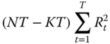
which follows a ![]() with
with ![]() if the underlying hypotheses of the within model are relevant.
if the underlying hypotheses of the within model are relevant.
4.3 Tests for Serial Correlation
A model with individual effects has composite errors that are serially correlated by definition. The presence of the time‐invariant error component gives rise to serial correlation that does not die out over time; thus standard tests applied on pooled data usually end up rejecting the null of spherical residuals. There may also be serial correlation of the time‐decaying kind in the idiosyncratic error terms, e.g., as an AR(1) process. By “testing for serial correlation” we mean testing for this latter kind of dependence.
For these reasons, the subjects of testing for individual error components and for serially correlated idiosyncratic errors are closely related. In particular, simple (marginal) tests for one direction of departure from the hypothesis of spherical errors usually have power against the other one: in case it is present, they are substantially biased toward rejection. Joint tests are correctly sized and have power against both directions but usually do not give any information about which one actually caused rejection. Conditional tests for serial correlation that take into account the error components are correctly sized under presence of both departures from sphericity and have power only against the alternative of interest. While most powerful if correctly specified, the latter, based on the likelihood framework, are crucially dependent on normality and homoscedasticity of the errors.
In plm a number of joint, marginal, and conditional ML‐based tests are provided, plus some semi‐parametric alternatives that are robust versus heteroscedasticity and free from distributional assumptions.
More tests can be obtained by comparing nested models, in a likelihood ratio test framework, or by restriction on a more general model, in the Wald test framework.
4.3.1 Unobserved Effects Test
The unobserved effects test à la Wooldridge (see Wooldridge, 2002, 10.4.4), is a semi‐parametric test for the null hypothesis that ![]() , i.e., that there are no unobserved effects in the residuals. Given that under the null, the covariance matrix of the residuals for each individual is diagonal, the test statistic is based on the average of elements in the upper (or lower) triangle of its estimate, diagonal excluded:
, i.e., that there are no unobserved effects in the residuals. Given that under the null, the covariance matrix of the residuals for each individual is diagonal, the test statistic is based on the average of elements in the upper (or lower) triangle of its estimate, diagonal excluded: ![]() (where
(where ![]() are the pooled OLS residuals), which must be “statistically close” to zero under the null, scaled by its standard deviation:
are the pooled OLS residuals), which must be “statistically close” to zero under the null, scaled by its standard deviation:
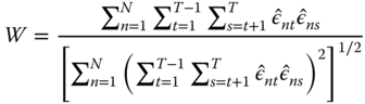
This test is (![]() ‐) asymptotically distributed as a standard normal regardless of the distribution of the errors. It does also not rely on homoscedasticity.
‐) asymptotically distributed as a standard normal regardless of the distribution of the errors. It does also not rely on homoscedasticity.
It has power both against the standard random effects specification, where the unobserved effects are constant within every group, as well as against any kind of serial correlation. As such, it “nests” both individual effects and serial correlation tests, trading some power against more specific alternatives in exchange for robustness.
While not rejecting the null favors the use of pooled OLS, rejection may follow from serial correlation of different kinds, and in particular, quoting Wooldridge (2002, 10.4.4), “should not be interpreted as implying that the random effects error structure must be true”.
4.3.2 Score Test of Serial Correlation and/or Individual Effects
The Wooldridge testing procedure will detect very general forms of persistence in the errors but give few directions toward a finer specification. If one is willing to make more specific parametric hypotheses, a maximum likelihood approach will allow to detect the features of persistence in a finer way.
The random effects model can be extended to having idiosyncratic errors that follow an autoregressive process of order 1 (AR(1)):
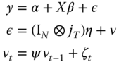
where the now familiar hypotheses of the random effects model apply, i.e., individual effects ![]() are independent of both the regressors and the idiosyncratic errors
are independent of both the regressors and the idiosyncratic errors ![]() . Moreover, normality is assumed for both error components.
. Moreover, normality is assumed for both error components.
The specification analysis of the above model requires telling apart the time‐invariant individual effects from the time‐decaying persistence due to the AR(1) component. As observed, the presence of individual effects may affect tests for serial correlation and vice versa. Several alternative strategies can be used, based on the following tools:
- a joint test, which has power against both alternatives,
- marginal tests, testing the null hypothesis of no serial correlation while maintaining the hypothesis of no individual effects under both the null and the alternative hypothesis,
- locally robust tests, i.e., marginal tests with a correction that makes them robust to local deviations from the maintained hypothesis,
- conditional test, i.e., testing the null hypothesis of no serial correlation, the hypothesis of the presence of individual effects being maintained under both the null and the alternative hypothesis.
The advantage of the robust tests is that the unconstrained model (RE‐AR(1) for random effect model with first‐order auto‐regressive errors) need not be estimated.
Baltagi and Li (1991) and Baltagi and Li (1995) proposed a joint test of no serial correlation and no individual effects. The test statistic is:
with ![]() and
and ![]() ,
, ![]() being the OLS residuals.
being the OLS residuals.
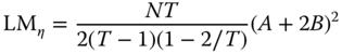
Baltagi and Li (1995) also proposed a marginal test of serial correlation, the maintained hypothesis being the absence of individual effects:

Symmetrically, the marginal test of individual effects, with the maintained hypothesis of no serial correlation is simply the Breusch‐Pagan test:

They also proposed a conditional test of serial correlation, the maintained hypothesis being the presence of individual effects. This latter test (![]() in the original paper) is based on the residuals of the random effect model estimated by the maximum likelihood method. Under the null of serially uncorrelated errors, the test turns out to be identical for both the alternative of AR(1) and MA(1) processes.
in the original paper) is based on the residuals of the random effect model estimated by the maximum likelihood method. Under the null of serially uncorrelated errors, the test turns out to be identical for both the alternative of AR(1) and MA(1) processes.
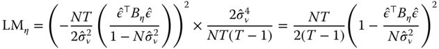
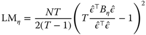
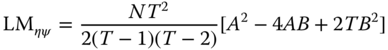
Bera et al. (2001) derive locally robust tests both for individual random effects and for first‐order serial correlation in residuals as “corrected” versions of the standard LM test ![]() and
and ![]() . They write respectively:
. They write respectively:
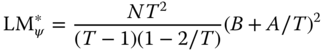
and
While still dependent on normality and homoscedasticity, these are robust to local departures from the hypotheses of, respectively, no serial correlation or no individual effects. Although suboptimal, these tests may help detecting the right direction of the departure from the null, thus complementing the use of joint tests. Moreover, being based on pooled OLS residuals, the BSY tests are computationally far less demanding than the conditional test of Baltagi and Li (1995).
On the other hand, the statistical properties of these locally corrected tests are inferior to those of the non‐corrected counterparts when the latter are correctly specified. If there is no serial correlation, then the optimal test for random effects is the likelihood‐based LM test of Breusch and Pagan (with refinements by Honda, see plmtest), while if there are no individual effects, the optimal test for serial correlation is the Breusch‐Godfrey test. If the presence of a random effect is taken for granted, then the optimal test for serial correlation is the likelihood‐based conditional LM test of Baltagi and Li (1995) (see pbltest).
4.3.3 Likelihood Ratio Tests for AR(1) and Individual Effects
Likelihood ratio (LR) tests for restrictions are based on the likelihoods from the general and the restricted model. The test statistic is simply twice the difference of the values of the log‐likelihood function:
where ![]() is the full vector of parameter estimates from the unrestricted model and
is the full vector of parameter estimates from the unrestricted model and ![]() from the restricted one, and
from the restricted one, and ![]() is the number of restrictions.
is the number of restrictions.
A likelihood ratio test for serial correlation in the idiosyncratic residuals can be done, in general, as a nested models test comparing the model with spherical idiosyncratic residuals with the more general alternative featuring AR(1) residuals. If both estimated models allow for random effects, then the test will become conditional on the latter feature.
Thus,
and symmetrically for ![]() .
.
4.3.4 Applying Traditional Serial Correlation Tests to Panel Data
A general testing procedure for serial correlation in fixed effects (FE), random effects (RE), and pooled‐OLS panel models alike can be based on considerations in (Wooldridge, 2002, 10.7.2). For the random effects model, Wooldridge (2002) observes that under the null of homoscedasticity and no serial correlation in the idiosyncratic errors, the residuals from the quasi‐demeaned regression must be spherical as well. Else, as the individual effects are wiped out in the demeaning, any remaining serial correlation must be due to the idiosyncratic component. Hence, a simple way of testing for serial correlation is to apply a standard serial correlation test to the quasi‐demeaned model. The same applies in a pooled model, w.r.t.the original data.
The FE case is different. It is well known that if the original model's errors are uncorrelated, then FE residuals are negatively serially correlated, with ![]() for each
for each ![]() (see Wooldridge, 2002, 10.5.4). This correlation clearly dies out as
(see Wooldridge, 2002, 10.5.4). This correlation clearly dies out as ![]() increases, so this kind of AR test is applicable to within model objects only for
increases, so this kind of AR test is applicable to within model objects only for ![]() “sufficiently large”. Baltagi and Li (1995) derive a basically analogous
“sufficiently large”. Baltagi and Li (1995) derive a basically analogous ![]() ‐asymptotic test for first‐order serial correlation in a FE panel model as a Breusch‐Godfrey LM test on within residuals (see Baltagi and Li, 1995, par. 2.3 and formula 12). They also observe that the test on within residuals can be used for testing on the RE model, as “the within transformation wipes out the individual effects, whether fixed or random.” Generalizing the Durbin‐Watson test to FE models by applying it to fixed effects residuals is documented in Bhargava et al. (1982). On the converse, in short panels the test gets severely biased toward rejection (or, as the induced correlation is negative, toward acceptance in the case of the one‐sided Durbin‐Watson test with
‐asymptotic test for first‐order serial correlation in a FE panel model as a Breusch‐Godfrey LM test on within residuals (see Baltagi and Li, 1995, par. 2.3 and formula 12). They also observe that the test on within residuals can be used for testing on the RE model, as “the within transformation wipes out the individual effects, whether fixed or random.” Generalizing the Durbin‐Watson test to FE models by applying it to fixed effects residuals is documented in Bhargava et al. (1982). On the converse, in short panels the test gets severely biased toward rejection (or, as the induced correlation is negative, toward acceptance in the case of the one‐sided Durbin‐Watson test with alternative set to 'greater'). See below for a serial correlation test applicable to “short” FE panel models.
As observed above, applying the pbgtest and pdwtest functions to an FE model is appropriate only if the time dimension is long enough. In the frequent case of ”short” panels, one of the two testing procedures due to Wooldridge (2002) and described in the next section should be used instead.
4.3.5 Wald Tests for Serial Correlation using within and First‐differenced Estimators
4.3.5.1 Wooldridge's within‐based Test
Due to the demeaning procedure, under the null of no serial correlation in the errors, the residuals of an FE model must be negatively serially correlated, with ![]() for each
for each ![]() . Wooldridge suggests basing a test for this null hypothesis on a pooled regression of FE residuals on their first lag:
. Wooldridge suggests basing a test for this null hypothesis on a pooled regression of FE residuals on their first lag:
Rejecting the restriction ![]() makes us conclude against the original null of no serial correlation.
makes us conclude against the original null of no serial correlation.
The function carrying out this procedure estimates the FE model, retrieves residuals, then estimates an auxiliary (pooled) AR(1) model, and tests the above‐mentioned restriction on ![]() . Internally, a heteroscedasticity‐ and autocorrelation‐consistent covariance matrix (
. Internally, a heteroscedasticity‐ and autocorrelation‐consistent covariance matrix (vcovHC, see next chapter) is used, as originally prescribed. The test is applicable to any FE panel model and in particular to “short” panels with small ![]() and large
and large ![]() .
.
4.3.5.2 Wooldridge's First‐difference‐based Test
In the context of the first difference model, Wooldridge (2002, 10.6.3) proposes a serial correlation test that can also be seen as a specification test to choose the most efficient estimator between fixed effects (within) and first difference (FD).
The starting point is the observation that if the idiosyncratic errors of the original model ![]() are uncorrelated, the errors of the (first) differenced model
are uncorrelated, the errors of the (first) differenced model ![]() will be correlated, with
will be correlated, with ![]() , while any time‐invariant effect is wiped out in the differencing. So a serial correlation test for models with individual effects of any kind can be based on estimating the auxiliary model
, while any time‐invariant effect is wiped out in the differencing. So a serial correlation test for models with individual effects of any kind can be based on estimating the auxiliary model
and testing the restriction ![]() , corresponding to the null of no serial correlation in the original model. Drukker (2003) provides Monte Carlo evidence of the good empirical properties of the test.
, corresponding to the null of no serial correlation in the original model. Drukker (2003) provides Monte Carlo evidence of the good empirical properties of the test.
On the other extreme (see Wooldridge, 2002, 10.6.1), if the differenced errors are uncorrelated, then ![]() is a random walk. In this latter case, the most efficient estimator is the first difference (FD) one; in the former case, it is the fixed effects one (within).
is a random walk. In this latter case, the most efficient estimator is the first difference (FD) one; in the former case, it is the fixed effects one (within).
4.4 Tests for Cross‐sectional Dependence
Next to the more familiar issue of serial correlation, a growing body of literature has been dealing with cross‐sectional dependence in panels, which can arise, e.g., if individuals respond to common shocks (as in common factor models) or if spatial diffusion processes are present, relating individuals in a way depending on a measure of distance (as in spatial models).
If cross‐sectional dependence is present, the consequence is, at a minimum, inefficiency of the usual estimators and invalid inference when using the standard covariance matrix. This is the case, for example, in unobserved effects models when cross‐sectional dependence is due to an unobservable factor structure but with factors uncorrelated with the regressors. In this case the within or RE are still consistent, although inefficient (see De Hoyos and Sarafidis, 2006). If the unobserved factors are correlated with the regressors, which can seldom be ruled out, consequences are more serious: the estimators will be inconsistent.
4.4.1 Pairwise Correlation Coefficients
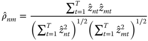
Correlation in the cross‐section can take very diverse shapes. The most common testing procedures are based on considering the population of all possible pairwise correlations between pairs of distinct individual units, estimating each one independently, by exploiting the time dimension of the data, and then calculating some synthetic measure or test statistic. The basic tool for assessing pairwise correlation between individual units ![]() and
and ![]() for a double‐indexed vector
for a double‐indexed vector ![]() is the product‐moment correlation coefficient, defined as
is the product‐moment correlation coefficient, defined as
A descriptive assessment of the degree of cross‐sectional correlation in the given sample can then be based on the average of individual correlation coefficients: ![]() . If individual correlations are some positive and some negative, this solution has the problem that coefficients with different signs compensate, yielding a statistic that underestimates the true level of dependence in the data. Therefore, another common procedure is to average the absolute values of individual coefficients:
. If individual correlations are some positive and some negative, this solution has the problem that coefficients with different signs compensate, yielding a statistic that underestimates the true level of dependence in the data. Therefore, another common procedure is to average the absolute values of individual coefficients: ![]() .
.
4.4.2 CD‐type Tests for Cross‐sectional Dependence
A number of statistics for testing the null hypothesis of no cross‐sectional dependence in model errors can be based on ![]() . The function
. The function pcdtest implements both the calculation of ![]() and
and ![]() , and a family of cross‐sectional dependence tests that can be applied in different settings, ranging from those where
, and a family of cross‐sectional dependence tests that can be applied in different settings, ranging from those where ![]() grows large with
grows large with ![]() fixed to “short” panels with a big
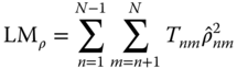
fixed to “short” panels with a big ![]() dimension and a few time periods. All are based on (transformations of) the product‐moment correlation coefficient of a model's residuals, defined as above. The Breusch‐Pagan LM test, based on the squares of
dimension and a few time periods. All are based on (transformations of) the product‐moment correlation coefficient of a model's residuals, defined as above. The Breusch‐Pagan LM test, based on the squares of ![]() , is valid for
, is valid for ![]() with
with ![]() fixed:
fixed:
where in the case of an unbalanced panel only pairwise complete observations are considered, and ![]() with
with ![]() being the number of observations for individual
being the number of observations for individual ![]() ; else, if the panel is balanced,
; else, if the panel is balanced, ![]() for each
for each ![]() . The test is distributed as
. The test is distributed as ![]() . It is inappropriate whenever the
. It is inappropriate whenever the ![]() dimension is “large.” A scaled version, applicable also if
dimension is “large.” A scaled version, applicable also if ![]() and then
and then ![]() (as in some pooled time series contexts), is defined as:
(as in some pooled time series contexts), is defined as:
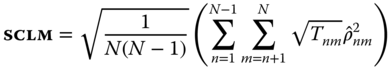
and distributed as a standard normal.
Pesaran's (2004) CD test

based on ![]() without squaring (also distributed as a standard Normal) is appropriate both for
without squaring (also distributed as a standard Normal) is appropriate both for ![]() ‐ and
‐ and ![]() ‐asymptotics. It has good properties in samples of any practically relevant size and is robust to a variety of settings. The only big drawback is that the test loses power against the alternative of cross‐sectional dependence if the average correlation is zero, even if individual coefficients are non‐zero. Such a situation is not uncommon and can arise for example in the presence of an unobserved factor structure with factor loadings averaging zero, that is, where some units react positively to common shocks, others negatively. Another case where the test will lose power is if the data are cross‐sectionally demeaned, or when the model contains time‐specific dummies (see Sarafidis and Wansbeek, 2012, p. 27). In these instances, the absolute correlation coefficient
‐asymptotics. It has good properties in samples of any practically relevant size and is robust to a variety of settings. The only big drawback is that the test loses power against the alternative of cross‐sectional dependence if the average correlation is zero, even if individual coefficients are non‐zero. Such a situation is not uncommon and can arise for example in the presence of an unobserved factor structure with factor loadings averaging zero, that is, where some units react positively to common shocks, others negatively. Another case where the test will lose power is if the data are cross‐sectionally demeaned, or when the model contains time‐specific dummies (see Sarafidis and Wansbeek, 2012, p. 27). In these instances, the absolute correlation coefficient ![]() is likely to turn out much bigger than
is likely to turn out much bigger than ![]() .
.
4.4.3 Testing Cross‐sectional Dependence in a pseries
Next to testing for cross‐sectional correlation in model residuals, tests in the CD family can be employed in preliminary statistical assessments as well, in order to determine whether the dependent and explanatory variables show any correlation to begin with. To this end, the pcdtest function has a pseries method, meaning that it can be fed a pseries object as well. One can either calculate the descriptive statistics ![]() and
and ![]() or resort to a formal test.
or resort to a formal test.