
Chapter 10
Spatial Panels
10.1 Spatial Correlation
If the cross‐sectional dimension of a dataset has any form of ordering, or if a distance is defined over each pair of observations (here: spatial units), one can use spatial methods to account for the possibility that correlation be stronger between “nearby” ones. The most commonly used definitions of proximity are either distance‐ or neighborhood‐related. Neighborhood depends on the spatial units being arranged in a topological space on a regular or irregular grid, an example of the latter being state or regional borders in geography.1 On the subject, see Anselin (1988, Ch. 3).
This subject is most relevant in nonrandom samples such as countries within a geographical region, or regions within one country; but spatial methods can also be employed wherever some kind of distance between observations is defined, be it in a geographic space or perhaps in an economic, demographic, or psychological one. Hence spatial methods, although more common in the former context, can be relevant in random samples too, such as, e.g., in household surveys.
10.1.1 Visual Assessment
Correlation in bidimensional space can be multifaceted, and in some ways more complicated to assess than correlation in time, which has a single dimension and often an obvious direction. Therefore, preliminary data analysis based on visual assessments, while always important and perhaps underutilized in econometric practice (Kleiber and Zeileis, 2008), is all the more useful in a spatial context. In the first part of this section we present an example of visual assessment of spatial correlation drawing on R's map plotting facilities; next, we proceed to formal statistical tests.
10.1.2 Testing for Spatial Dependence
One first issue when confronted with spatially referenced data is to determine whether spatial dependence exists, i.e., whether “nearby” units (according to the chosen metric) are more correlated than distant ones. The raw data are tested for spatial dependence in order to inform and justify the use of spatial estimation methods; then, after estimation, the residuals are tested again to determine whether the model has been able to effectively account for the spatial features of the process at hand.
10.1.2.1 CD p Tests for Local Cross‐sectional Dependence
A very flexible way of assessing whether dependence in the cross‐section of a panel dataset is spatially related goes through a particularization of the CD test for general cross‐sectional dependence described in Chapter . The latter is in principle completely a‐spatial, being based on a scaled average of the pairwise correlation coefficients ![]() between observations (or residuals). Still, the CD can be restricted to those pairs of observations satisfying one given criterion: most frequently, a contiguity‐based neighborhood one but also that distance be under a given cutoff level.
between observations (or residuals). Still, the CD can be restricted to those pairs of observations satisfying one given criterion: most frequently, a contiguity‐based neighborhood one but also that distance be under a given cutoff level.
The local variant of the CD test, called ![]() test (Pesaran, 2004), takes into account an appropriate subset of neighboring cross‐sectional units to check the null of no cross‐sectional dependence against the alternative of local cross‐sectional dependence, i.e., dependence between neighbors only. To do so, the pairs of neighboring units are selected by means of a binary proximity matrix, in which zeros correspond to pairs of observations that are not neighbors. The latter is used for discarding the correlation coefficients relative to pairs of observations that are not neighbors in computing the CD statistic. The test is then defined as:
test (Pesaran, 2004), takes into account an appropriate subset of neighboring cross‐sectional units to check the null of no cross‐sectional dependence against the alternative of local cross‐sectional dependence, i.e., dependence between neighbors only. To do so, the pairs of neighboring units are selected by means of a binary proximity matrix, in which zeros correspond to pairs of observations that are not neighbors. The latter is used for discarding the correlation coefficients relative to pairs of observations that are not neighbors in computing the CD statistic. The test is then defined as:

where ![]() is the
is the ![]() ‐th element of the
‐th element of the ![]() ‐th order proximity matrix, so that if any pair
‐th order proximity matrix, so that if any pair ![]() are not neighbors,
are not neighbors, ![]() and
and ![]() is eliminated from the summation; and
is eliminated from the summation; and ![]() is the number of time series observations in common between individuals
is the number of time series observations in common between individuals ![]() and
and ![]() (
(![]() if the panel is balanced).2
if the panel is balanced).2
The same procedure can be applied to the LM and SCLM tests described in section 4.3.1. The local version of either test can be computed supplying an ![]() matrix (of any type coercible to
matrix (of any type coercible to logical), providing information on whether any pair of observations are neighbors or not, to the w argument of pcdtest. If w is supplied, only neighboring pairs will be used in computing the test; else, w will default to NULL, and all observations will be used. The matrix needs not really be binary, so commonly used “row‐standardized” matrices can be employed as well: it is enough that neighboring pairs correspond to nonzero elements in w3.
10.1.2.2 The Randomized W Test
The ![]() test is flexible and well behaved in small samples; moreover it does not suffer the biggest drawback of its global sibling, which does not have any power under zero‐mean dependence and therefore cannot be employed, for example, on cross‐sectionally demeaned data – or equivalently on the residuals of a model containing time fixed effects. Nevertheless, it does not tolerate serial correlation and can be sensitive to non‐spatial types of dependence. In fact, if cross‐sectional dependence of the non‐spatial type is present and a
test is flexible and well behaved in small samples; moreover it does not suffer the biggest drawback of its global sibling, which does not have any power under zero‐mean dependence and therefore cannot be employed, for example, on cross‐sectionally demeaned data – or equivalently on the residuals of a model containing time fixed effects. Nevertheless, it does not tolerate serial correlation and can be sensitive to non‐spatial types of dependence. In fact, if cross‐sectional dependence of the non‐spatial type is present and a ![]() test is performed, it will be based on a subset of spatially related pairs from a population of correlated ones; it is therefore likely to yield a false positive result (a type I error) favoring spatial dependence.
test is performed, it will be based on a subset of spatially related pairs from a population of correlated ones; it is therefore likely to yield a false positive result (a type I error) favoring spatial dependence.
The idea underlying the ![]() test, that not all pairs of neighbors are correlated but only those in a specific spatial relationship are and that the latter are identified through the
test, that not all pairs of neighbors are correlated but only those in a specific spatial relationship are and that the latter are identified through the ![]() matrix, gives rise to another testing procedure that is remarkably robust to all the above confounding features. The RW test of Millo (2017a) employs a permutation procedure to produce a large number of randomized neighborhood matrices and then compares the
matrix, gives rise to another testing procedure that is remarkably robust to all the above confounding features. The RW test of Millo (2017a) employs a permutation procedure to produce a large number of randomized neighborhood matrices and then compares the ![]() statistic under the true spatial ordering with the population of those under the randomized ones. If spatial dependence is absent, the observations must be exchangeable in the cross‐section: then, the true
statistic under the true spatial ordering with the population of those under the randomized ones. If spatial dependence is absent, the observations must be exchangeable in the cross‐section: then, the true ![]() will not take an extreme value with respect to the randomization‐based ones, and the null hypothesis of no spatial dependence will hold. As usual, the share of randomized statistics more extreme than the true one will be the pseudo‐
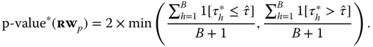
will not take an extreme value with respect to the randomization‐based ones, and the null hypothesis of no spatial dependence will hold. As usual, the share of randomized statistics more extreme than the true one will be the pseudo‐![]() of the test. In the majority of situations, the alternative hypothesis is of positive spatial dependence. In this case a one‐tailed test will be appropriate. Given a panel‐indexed vector
of the test. In the majority of situations, the alternative hypothesis is of positive spatial dependence. In this case a one‐tailed test will be appropriate. Given a panel‐indexed vector ![]() , call
, call ![]() the randomized statistic from the
the randomized statistic from the ![]() ‐th draw, with
‐th draw, with ![]() ; and
; and ![]() the one under the true W. If the alternative is positive spatial dependence, the pseudo‐
the one under the true W. If the alternative is positive spatial dependence, the pseudo‐![]() of the one‐tailed
of the one‐tailed ![]() test is then
test is then

where ![]() is the indicator function. The null of no spatial dependence in
is the indicator function. The null of no spatial dependence in ![]() would be rejected at, say, 5% significance if
would be rejected at, say, 5% significance if ![]() , meaning that the actual
, meaning that the actual ![]() value is more extreme than the 95th quantile of the distribution of randomized values.
value is more extreme than the 95th quantile of the distribution of randomized values.
Negative spatial autocorrelation is less common in empirical practice but can be relevant, e.g., in the description of competitive processes (see Griffith and Arbia, 2010; Elhorst and Zigova, 2014). In this case it may happen that the distribution of randomized statistics be shifted in the opposite direction by positive global dependence so that the value of the true test statistic be less extreme, and the one‐tailed procedure would not work. A two‐tailed test is then needed, which is easily accomplished by taking absolute values and cross‐sectionally demeaning the data so that the average of the factors, and hence the average global correlation, is re‐centered on zero:

To take heed of possible asymmetries in the (re‐centered) distribution of randomized statistics, one can go the safest way employing the asymmetric version of the test:
10.2 Spatial Lags
The basic tool of spatial econometrics is the definition of a spatial lag. Given an observation and a distance metric, the spatial lag of that observation is usually defined as some kind of weighted average of the observations that are considered “near” to it according to the given metric: ![]() . Either a distance or a neighborhood matrix is commonly employed to provide the weights. In the neighborhood case, for each pair of observations
. Either a distance or a neighborhood matrix is commonly employed to provide the weights. In the neighborhood case, for each pair of observations ![]() , the matrix will have an element
, the matrix will have an element ![]() if the two are neighbors, i.e., if they share a common border like Germany and Austria (first‐order neighborhood) or if there are at most
if the two are neighbors, i.e., if they share a common border like Germany and Austria (first‐order neighborhood) or if there are at most ![]() other observations separating them (
other observations separating them (![]() ‐th order neighborhood), so that Italy and Germany are second‐order neighbors. In the distance‐based case, the generic element will be dependent on some inverse function of the distance
‐th order neighborhood), so that Italy and Germany are second‐order neighbors. In the distance‐based case, the generic element will be dependent on some inverse function of the distance ![]() between them, usually the reciprocal:
between them, usually the reciprocal: ![]() . It is customary to set a cutoff point at some distance
. It is customary to set a cutoff point at some distance ![]() beyond which one does not expect any influence to be present so that
beyond which one does not expect any influence to be present so that ![]() if
if ![]() 4. In both cases, it is customary to standardize
4. In both cases, it is customary to standardize ![]() so that the rows sum to one:
so that the rows sum to one: ![]() . Then, for each
. Then, for each ![]() ,
, ![]() will contain, respectively, the simple average of values in neighboring locations or a distance‐weighted average of all
will contain, respectively, the simple average of values in neighboring locations or a distance‐weighted average of all ![]() for which
for which ![]() .
.
In all of the following, we will refer to the simpler neighborhood‐based definition of proximity. All techniques illustrated in this chapter are nevertheless applicable as well in the case of distance‐based weights. The spatial weights matrix can be based on definitions of distance not based on geographical position but defined instead in some other kind of space, like e.g., one where dimensions are corresponding to some set of economic or demographic or psychological characteristics. The technical aspects of estimation do not vary with respect to the case of geographical distance, or neighborhood, as long as the fundamental hypothesis of exogeneity of ![]() holds. One desirable feature of geographic space is that it is exogenous, unlike, e.g., bilateral (contemporaneous) trade‐based weights in a model of international commerce, which would be generated inside the same economic system to be modeled.
holds. One desirable feature of geographic space is that it is exogenous, unlike, e.g., bilateral (contemporaneous) trade‐based weights in a model of international commerce, which would be generated inside the same economic system to be modeled.
It is important to recall that the hypothesis of exogenous and time‐invariant ![]() will be maintained throughout this chapter. Spatial lags in a panel setting can be written compactly in vector form stacking observations by time first, in the now‐standard notation, as
will be maintained throughout this chapter. Spatial lags in a panel setting can be written compactly in vector form stacking observations by time first, in the now‐standard notation, as ![]() . The concept of spatial lag has some analogies with the familiar time lag but also important differences, the most important one being that while time is directed, space is generally not; hence the idea of predeterminedness and the fact that usually (although not always) the past is expected to influence the future but not vice versa do not apply. Dependence in space is usually circular, and the influence from “nearby” observations gives rise to feedback effects that importantly affect estimation. In particular, as will be clear in the following, a spatial lag of the dependent variable is endogenous by construction, and a model including it will require more sophisticated techniques than (ordinary or generalized) least squares in order to be consistently estimated.
. The concept of spatial lag has some analogies with the familiar time lag but also important differences, the most important one being that while time is directed, space is generally not; hence the idea of predeterminedness and the fact that usually (although not always) the past is expected to influence the future but not vice versa do not apply. Dependence in space is usually circular, and the influence from “nearby” observations gives rise to feedback effects that importantly affect estimation. In particular, as will be clear in the following, a spatial lag of the dependent variable is endogenous by construction, and a model including it will require more sophisticated techniques than (ordinary or generalized) least squares in order to be consistently estimated.
10.2.1 Spatially Lagged Regressors
Suppose that the need to account for space in the specification has been established either a priori, in the economic model, or because spatial dependence has been detected in the data or in the residuals of an estimated model.
One first way to consider the influence of neighboring spatial units is to take into account spatial lags of the explanatory variables. The economic meaning of spatially lagged regressors is to account for explicit spatial influences from relevant explanatory variables in nearby spatial units. Spatial lags ![]() can easily be added to the specification and, provided
can easily be added to the specification and, provided ![]() was exogenous to begin with, pose no additional problem in estimation of this model.
was exogenous to begin with, pose no additional problem in estimation of this model.
As a first example of augmenting a model with a spatial lag, let us consider the case of a spatially lagged regressor representing (if ![]() is row‐standardized) the average of
is row‐standardized) the average of ![]() at neighboring locations.
at neighboring locations.
10.2.2 Spatially Lagged Dependent Variables
A more direct, although much more problematic, way of incorporating spatial structure in an econometric model is through inclusion of spatial lags of the dependent variable. The model is then:
where ![]() is the
is the ![]() spatial weights matrix of known constants whose diagonal elements are set to zero, and
spatial weights matrix of known constants whose diagonal elements are set to zero, and ![]() is the corresponding spatial parameter.
is the corresponding spatial parameter.
This is called the spatial lag model proper. From a theoretical viewpoint, it is appropriate whenever one expects the outcome of one observation to influence the outcomes of neighboring ones, such as, e.g., for the spreading of a disease, where one unit being positive has a direct effect on the likelihood of neighboring units to be so too.
Another example is if (within‐period) strategic interaction is expected to happen, e.g., each country takes the tax rates of neighbors into account in setting its own and may react within the same time period, as in Franzese and Hays (2006). In this case, one might expect positive spatial correlation. In a microeconomic setting, the effect of a spatial lag term could be expected to turn out positive is in copycatting behavior, when e.g., buying a product sparks imitation hereby raising the propensity of neighbors to follow suit. A negative spatial lag can instead be consistent with the idea of free riding: if one can reap advantage from the actions of neighbors through some kind of externality, then this will lower his or her own effort: an example is labor market training in the European Union, where trained labor can easily commute across borders (Franzese and Hays, 2008).
Spatial‐lag‐type dependence has been evocatively termed “substantial” (Franzese and Hays, 2007) as opposed to spatial error dependence, which in the same context is described as “nuisance,” to be controlled for the sake of precision in estimation but devoid of theoretical meaning. This is not necessarily true, as spatial error dependence can have substantial meaning too, for example in the context of economic shock diffusion (see e.g. Holly et al., 2010), and can be a subject of the analysis in its own right.
The spatial lag process, and by extension the model with a spatial lag plus regressors, is universally known by the acronym SAR, for “spatially autoregressive.” The ![]() term is inherently endogenous; in a reduced form, the model becomes nonlinear:
term is inherently endogenous; in a reduced form, the model becomes nonlinear:
so that maximum likelihood estimation (ML) is called for. Only as a very first approximation, it can be of interest to estimate the so‐called “spatial OLS”.
10.2.2.1 Spatial OLS
Ordinary least squares estimation is consistent, under the usual exogeneity conditions on ![]() , for models with spatially lagged regressors, in which case it is also efficient provided that the standard hypotheses of homoscedasticity and incorrelation hold; in fact, adding
, for models with spatially lagged regressors, in which case it is also efficient provided that the standard hypotheses of homoscedasticity and incorrelation hold; in fact, adding ![]() may eliminate the spatial correlation in error terms and effectively make OLS the efficient estimator. Even in the case of the spatial error model, OLS remain consistent, although inefficient, for
may eliminate the spatial correlation in error terms and effectively make OLS the efficient estimator. Even in the case of the spatial error model, OLS remain consistent, although inefficient, for ![]() .
.
As a first approximation, and in cases where ML and GM are problematic (one for all, dynamic panels), the so‐called spatial‐OLS method has been advocated: adding the spatial lag of the dependent variable ![]() to the right‐hand side regressors. This solution is in general not advisable because
to the right‐hand side regressors. This solution is in general not advisable because ![]() is endogenous by construction, and therefore the estimator is hopelessly biased; yet simulation studies have shown how the magnitude of the bias can be limited in real‐world cases, to the point of making this computationally simple solution relatively viable in some applied settings (see Franzese and Hays, 2007).
is endogenous by construction, and therefore the estimator is hopelessly biased; yet simulation studies have shown how the magnitude of the bias can be limited in real‐world cases, to the point of making this computationally simple solution relatively viable in some applied settings (see Franzese and Hays, 2007).
10.2.2.2 ML Estimation of the SAR Model
An appropriate way to estimate a SAR model, provided the errors ![]() are i.i.d. normal, is by ML. Let us start from the cross‐sectional case where
are i.i.d. normal, is by ML. Let us start from the cross‐sectional case where ![]() is
is ![]() and
and ![]() is a vector of length
is a vector of length ![]() . Denoting
. Denoting ![]() , the model becomes
, the model becomes ![]() so that
so that ![]() . Expressing the usual likelihood function of the linear model in terms of the transformed
. Expressing the usual likelihood function of the linear model in terms of the transformed ![]() requires adding the Jacobian of the transformation, i.e., the determinant of
requires adding the Jacobian of the transformation, i.e., the determinant of ![]() , therefore the log‐likelihood becomes:
, therefore the log‐likelihood becomes:
and this likelihood is to be optimized with respect to ![]() and
and ![]() , efficient optimization strategies having been outlined in the seminal book of Anselin (1988). The pure‐SAR panel case, pooling the data without any individual feature, just substitutes
, efficient optimization strategies having been outlined in the seminal book of Anselin (1988). The pure‐SAR panel case, pooling the data without any individual feature, just substitutes ![]() for
for ![]() ,
, ![]() for
for ![]() and
and ![]() so that it could be estimated with the
so that it could be estimated with the lagsarlm function from package spdep. Nevertheless, it is always preferable for computational reasons to resort to specific methods for spatial panels when available.
10.2.3 Spatially Correlated Errors
The other main specification in the literature, the spatial error, is instead appropriate when one expects the innovation relative to one observation to influence the outcomes of neighboring ones, as would be the case for an economic shock of some kind to a given region (fully) influencing the relevant dependent variable in that region and also propagating – with distance‐decaying intensity – toward nearby ones; or for a location‐related measurement error, by its nature affecting nearby observations in a similar way. Another reason for spatially correlated errors is misspecification resulting from the omission of a spatially correlated variable. This specification is called SEM, for “spatial error model”.
The model is then the familiar linear model with regressors:
where ![]() is a vector of spatially autocorrelated idiosyncratic errors that follows a spatial autoregressive process of the form
is a vector of spatially autocorrelated idiosyncratic errors that follows a spatial autoregressive process of the form
with ![]() as the spatial autoregressive parameter,
as the spatial autoregressive parameter, ![]() the spatial weights matrix and
the spatial weights matrix and ![]() . As can be seen, the SEM model is nothing but a linear model with a SAR process in the errors instead of in the response. The likelihood for the cross‐sectional SEM model is:
. As can be seen, the SEM model is nothing but a linear model with a SAR process in the errors instead of in the response. The likelihood for the cross‐sectional SEM model is:
where ![]() . As for the SAR case, pooling the data is accomplished by substituting
. As for the SAR case, pooling the data is accomplished by substituting ![]() to
to ![]() , the extended proximity matrix
, the extended proximity matrix ![]() for
for ![]() and
and ![]() .
.
It is typical in the literature to estimate either of the two specifications, SAR or SEM, although in principle they can be combined. The subject of choosing between the spatial lag and the spatial error models by means of diagnostic testing will be treated in the following; it should nevertheless be borne in mind that the specification of one or the other spatial model should always be informed by the a priori beliefs of the researcher and the economic model she postulates for the phenomenon at hand. In fact, while some empirical cases happen to be sufficiently clear‐cut for an exclusively data‐driven decision to be taken, most of the time model uncertainty – regarding the specification of regressors, of the neighborhood structure (the ![]() matrix), or that of the spatial process in either response or error – is so pervasive that one can hardly rely on statistical procedures alone in order to conduct a specification search.
matrix), or that of the spatial process in either response or error – is so pervasive that one can hardly rely on statistical procedures alone in order to conduct a specification search.
Nevertheless, from a diagnostic rather than modeling viewpoint, a general result is that the omission of a spatially correlated relevant regressor would show up as spatially correlated errors, and the same would happen for the omission of a spatially lagged dependent variable; much as would happen in time series data with omitted dynamics showing up in residual autocorrelation. Generality stops here, though, because while the symptoms of either neglected spatial lag or error processes are similar, the consequences on the properties of estimators are different already. In fact, an omitted spatial lag renders the estimator inconsistent, while an omitted spatial process in the error merely results in inefficiency and invalid inference.
10.3 Individual Heterogeneity in Spatial Panels
Cross‐sectional spatial specifications are readily extended to the case of a pooled panel dataset, as above, but in the case of spatial panels, just as in the general case, it becomes of primary interest to model heterogeneity and persistence at the individual level. Again, the most popular device is the inclusion of individual, time‐invariant effects in the model, and again the crucial distinction is whether said effects can be assumed independent from the model regressors or not. From a statistical viewpoint, the approach detailed in the previous chapters when speaking of non‐spatial panels is still valid, but there are also specific considerations to be made for spatial applications. For example, as the random effects hypothesis is considered consistent with sampling individuals from a potentially infinite population, some (Elhorst and Fréret (2009) for example) have dismissed its plausibility in spatial econometric contexts, where sampling most typically takes place over a fixed set of countries or regions.
Spatial methods are nevertheless of interest also in contexts much akin to random sampling. For one, applications on survey data can be devised where individual units are located into some non‐geographic space, defined by their attributes and a distance function. Among the geographically referenced data proper, the same random samples of firms or households can be located and recorded as points in the landscape (Bell and Bockstael, 2000). In this sense, the RiceFarms dataset is a good candidate for random effects: many locations with similar characteristics, plausibly drawn from the same distribution, although lacking latitude and longitude information, are grouped in a way that naturally defines a neighborhood. Another case, where this time data are located as points in geographical space, are the ever more popular spatial applications from experimental contexts in life sciences, of which we will see an example later in the chapter.
Moreover, from a computational viewpoint random effects turn out to be a more general case with respect to fixed effects.
10.3.1 Random versus Fixed Effects
As detailed in the previous chapters and recalled above, unobserved individual heterogeneity is dealt with in different ways depending on the statistical properties of the individual effects, the crucial distinction becoming whether one can assume them to be uncorrelated with the regressors or not. If uncorrelated, then individual effects can be considered as a component of the error term. If not, then the latter strategy leads to inconsistency; the individual effects will have to be estimated or, more frequently, eliminated by first differencing or time‐demeaning the data. In the spatial setting, the standard solution to the fixed effects case has long been time‐demeaning: in the framework of Elhorst (2003), fixed effects estimation of spatial panel models is accomplished as pooled ML estimation on time‐demeaned data. Nevertheless, Elhorst's procedure has been questioned by Anselin et al. (2008) because time‐demeaning alters the properties of the joint distribution of errors, introducing serial dependence. As it turns out, despite the misspecification of the likelihood, the only parameter affected is the variance of the error term, the other estimators remaining consistent.7
To solve the problem, Lee and Yu (2010a, 3.2) suggest either a different orthonormal transformation of the data, or an ex‐post correction of the estimated variance (see also Lee and Yu, 2012). For all this, ML estimation of spatial panel models with individual fixed effects is encompassed by the ML estimator for the pooled case, after a suitable transformation of the data and, in the case one uses the simpler within transformation, an appropriate ex‐post correction of the error variance estimate.
10.3.2 Spatial Panel Models with Error Components
While fixed effects estimation of spatial panels can be performed in the framework of the pooled spatial models, after transforming out the individual effects by a within transformation, treating the individual effects as random introduces substantial complications in the specification of the likelihood.
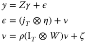
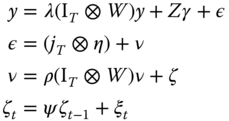
We consider a general static panel model that includes a spatial lag of the dependent variable and spatial autoregressive disturbances:
The disturbance vector is the sum of two terms:
![]() being the individual effect and
being the individual effect and ![]() a vector of spatially autocorrelated idiosyncratic errors that follow a spatial autoregressive process of the form
a vector of spatially autocorrelated idiosyncratic errors that follow a spatial autoregressive process of the form
with ![]() as the spatial autoregressive parameter,
as the spatial autoregressive parameter, ![]() the spatial weights matrix and
the spatial weights matrix and ![]() . The spatial weights matrices in the lag and the error term can differ (see the following).
. The spatial weights matrices in the lag and the error term can differ (see the following). ![]() is assumed non‐singular.
is assumed non‐singular.
10.3.2.1 Spatial Panels with Independent Random Effects
In a random effects specification, the unobserved individual effects are assumed uncorrelated with the other explanatory variables in the model and can therefore be safely treated as components of the error term.8 In this case, ![]() , and the error term can be rewritten as:
, and the error term can be rewritten as:
where ![]() . As a consequence, the composite error term becomes
. As a consequence, the composite error term becomes
and its variance‐covariance matrix is:
In deriving several Lagrange multiplier (LM) tests, Baltagi et al. (2003b) consider a panel data regression model that is a special case of the model presented above in that it does not include a spatial lag of the dependent variable. Elhorst (2003), Elhorst and Fréret (2009) define a taxonomy for spatial panel data models both under the fixed and the random effects assumptions. Following the typical distinction made in cross‐sectional models, they define the fixed as well as the random effects panel data versions of the spatial error and spatial lag models. However, unlike Case (1991), they do not consider a model including both the spatial lag of the dependent variable and a spatially autocorrelated error term. Therefore, the models reviewed in Elhorst (2003), Elhorst and Fréret (2009) can also be seen as special cases of this more general specification.
Following the treatment in Millo (2014), on which this part of the chapter is based, we label the combined model containing both a spatial lag and a spatial error process SAREM. (This is also often called ![]() , because of the two spatial autoregressive processes, one in the response and one in the errors.) If a random individual effect is also part of the composite error term, then we will add the suffix RE. Although SAR and SEM, combined with either FE or RE, are by far the most popular specifications, the literature has also dealt with different types of spatial diffusion processes in the errors other than the autoregressive one, most notably the spatial moving average.9 We do not consider them here.
, because of the two spatial autoregressive processes, one in the response and one in the errors.) If a random individual effect is also part of the composite error term, then we will add the suffix RE. Although SAR and SEM, combined with either FE or RE, are by far the most popular specifications, the literature has also dealt with different types of spatial diffusion processes in the errors other than the autoregressive one, most notably the spatial moving average.9 We do not consider them here.
10.3.2.2 Spatially Correlated Random Effects
A different specification for the disturbances was considered in Kapoor et al. (2007). They assume that spatial correlation applies to both the individual effects and the remainder error components. Although the two data‐generating processes look similar, they do imply different spatial spillover mechanisms governed by a different structure of the implied variance‐covariance matrix. In this case, commonly referred to as KKP, the composite disturbance term
follows a first‐order spatial autoregressive process of the form:
It follows that the variance‐covariance matrix of ![]() is:
is:
where ![]() is the typical variance‐covariance matrix of a one‐way error component model. The variance matrix in (10.5) is simpler than the one in (10.4), and therefore its inverse is easier to calculate, as will be discussed below. As Baltagi et al. (2013) observe, the economic meaning of the two models is also different: in the first model only the time‐varying components diffuse spatially; in the second, spatial spillovers too have a permanent component. Lee and Yu (2012, 2.4) illustrate the difference between this latter specification and
is the typical variance‐covariance matrix of a one‐way error component model. The variance matrix in (10.5) is simpler than the one in (10.4), and therefore its inverse is easier to calculate, as will be discussed below. As Baltagi et al. (2013) observe, the economic meaning of the two models is also different: in the first model only the time‐varying components diffuse spatially; in the second, spatial spillovers too have a permanent component. Lee and Yu (2012, 2.4) illustrate the difference between this latter specification and ![]() through the likelihood of the between model. We label this latter alternative specification
through the likelihood of the between model. We label this latter alternative specification ![]() , and its extension to including a spatial lag (see Mutl and Pfaffermayr, 2011)
, and its extension to including a spatial lag (see Mutl and Pfaffermayr, 2011) ![]() .
.
10.3.3 Estimation
To review the theory of maximum likelihood estimation of spatial panel models with random effects, we will start from models with a spatially lagged dependent variable, spatial error correlation, and a general covariance structure for the error, as described by Anselin (1988), without any panel structure (although it must be noted that in his book Anselin (1988) already considered a SEM panel with random effects, deriving the model likelihood, as a special case). Following Millo (2014), we will introduce random effects as just one particular type of error covariance structure, thus comprising spatial panels in Anselin's general framework.10
10.3.3.1 Spatial Models with a General Error Covariance
Maximum Likelihood estimation with a general error covariance matrix has been outlined in Magnus (1978) (see also Anselin et al., 2008). If the error ![]() is distributed as
is distributed as ![]() then the log‐likelihood is
then the log‐likelihood is
Particularizing this likelihood w.r.t. the case at hand, and adding a spatial filter if needed, provides a general framework for ML estimation of the models of interest. Anselin (1988), the classic reference on spatial econometric model estimation by ML, outlines the general procedure for a model with spatial lag, spatial errors, and possibly nonspherical residuals as follows. Let us restrict the analysis, for the moment, to one cross‐section and let our model be:

with ![]() and, in general,
and, in general, ![]() . Two special cases of this general model are often found in applied literature: if
. Two special cases of this general model are often found in applied literature: if ![]() one has the spatial autoregressive (SAR) model, while if
one has the spatial autoregressive (SAR) model, while if ![]() , the spatial (autoregressive) error (SEM) model. Both usually include the hypothesis of spherical remainder errors:
, the spatial (autoregressive) error (SEM) model. Both usually include the hypothesis of spherical remainder errors: ![]() . Introducing the now‐standard simplifying notation
. Introducing the now‐standard simplifying notation ![]() ,
, ![]() the model becomes:
the model becomes:

where ![]() are potentially different spatial weights matrices.11 If there exists
are potentially different spatial weights matrices.11 If there exists ![]() such that
such that ![]() and
and ![]() , and
, and ![]() is invertible, then
is invertible, then ![]() and the model (10.6) can be written as
and the model (10.6) can be written as
or, equivalently,
with ![]() a “well‐behaved” error.
a “well‐behaved” error.
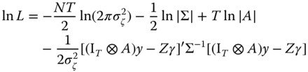
Still following Anselin, making the estimator operational requires the transformation from the unobservable ![]() to observables. Expressing the likelihood function in terms of
to observables. Expressing the likelihood function in terms of ![]() requires calculating the Jacobian of the transformation
requires calculating the Jacobian of the transformation ![]() . These determinants are to be added to the log‐likelihood, which becomes
. These determinants are to be added to the log‐likelihood, which becomes
where the difference w.r.t. the usual likelihood of the classic linear model is given by the terms of the Jacobian.12 The likelihood is thus a function of ![]() ,
, ![]() ,
, ![]() , and parameters in
, and parameters in ![]() .
.
It will be convenient for our purposes, and without loss of generality, to scale the overall errors' covariance writing it as ![]() (the latter expression is in fact more general, as it does not constrain the heteroscedastic error term
(the latter expression is in fact more general, as it does not constrain the heteroscedastic error term ![]() to be spatially lagged, through premultiplication by
to be spatially lagged, through premultiplication by ![]() , in its entirety. In our case, only the error covariance of the
, in its entirety. In our case, only the error covariance of the ![]() specification can be separated into a heteroscedastic error term and a spatial filter and therefore straightforwardly written as
specification can be separated into a heteroscedastic error term and a spatial filter and therefore straightforwardly written as ![]() , while the more common SEM specification cannot). This likelihood can be concentrated w.r.t.
, while the more common SEM specification cannot). This likelihood can be concentrated w.r.t.![]() and the error variance
and the error variance ![]() , by substituting
, by substituting ![]()

and a closed‐form GLS solution for ![]() and
and ![]() is available for any given set of spatial and other covariance parameters
is available for any given set of spatial and other covariance parameters

so that a two‐step procedure is possible that alternates optimization of the concentrated likelihood and GLS estimation. From here on, we explicitly consider the (balanced) panel structure of the data: ![]() individuals observed over
individuals observed over ![]() time periods.
time periods.
10.3.3.2 General Maximum Likelihood Framework
Building on the framework from Anselin (1988) outlined above, explicitly particularizing and operationalizing it with respect to a number of possible error covariance structures, all specifications outlined above can be estimated without the need to pre‐transform the data as has been customary in the literature since Elhorst (2003). Random effects will instead be considered as one feature of the errors' covariance, just like spatial (or, later on in the chapter, serial) correlation (see Millo, 2014). Considering the spatial dependence features together with all the other sources of heteroscedasticity and correlation instead of separating it clearly, as done in the original Anselin framework, has the advantage of keeping some components of the error term (most notably, the random effects) out of the spatial dependence, which can remain a feature of the idiosyncratic error only, in accordance with most applications in the literature; but also some clear computational disadvantages, as will be discussed below. We will also consider the alternative specification where the individual effects are lagged together with the idiosyncratic errors, as in Kapoor et al. (2007), which one can straightforwardly express in terms of Anselin's original expression ![]() , also extending the structure of
, also extending the structure of ![]() to include serial correlation. This latter will turn out to be easier to compute, especially on large examples.
to include serial correlation. This latter will turn out to be easier to compute, especially on large examples.
First we will discuss the combination of a spatial lag with any error covariance structure; then we will review the most significant among the latter; lastly we will give an example of operationalization through the use of analytical expressions for the inverse and determinant of the error covariance matrix ![]() .
.
Optimization will generally be subject to box constraints according to the following rules: the spatial lag and spatial errors coefficients ![]() and
and ![]() will be bounded between
will be bounded between ![]() and 1, where
and 1, where ![]() is the smallest characteristic root of
is the smallest characteristic root of ![]() ;13 the serial correlation coefficient will be constrained to the usual stationarity condition
;13 the serial correlation coefficient will be constrained to the usual stationarity condition ![]() and the variance ratio of the random effects
and the variance ratio of the random effects ![]() to be non‐negative.
to be non‐negative.
Spatial Lag
Although both the SAR and the SEM specifications are popular in the literature, estimation generally focuses on one effect only, and there are few applications allowing for both of them to be present in the estimated model, one notable exception being the pioneering work of Case (1991). It is nevertheless straightforward, at least as far as expressing the likelihood is concerned, to combine a spatial lag with any error structure, including spatial dependence ones.
The general likelihood for the spatial lag panel model combined with any error covariance structure ![]() is a panel version of (10.7):
is a panel version of (10.7):
The usual iterative procedure a la Oberhofer and Kmenta (1974) can be employed to obtain the maximum likelihood estimates. Starting from an initial value for the spatial lag parameter ![]() and the error covariance parameters, we obtain estimates for
and the error covariance parameters, we obtain estimates for ![]() and
and ![]() from the first‐order conditions:
from the first‐order conditions:
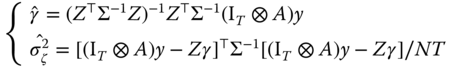
The likelihood can be concentrated and maximized with respect to the parameters in ![]() and
and ![]() . The estimated values thereof are then used to update the expression for
. The estimated values thereof are then used to update the expression for ![]() These steps are then repeated until convergence. In other words, for a specific
These steps are then repeated until convergence. In other words, for a specific ![]() the estimation can be operationalized by a two‐step iterative procedure that alternates between GLS (for
the estimation can be operationalized by a two‐step iterative procedure that alternates between GLS (for ![]() and
and ![]() ) and concentrated likelihood (for the remaining parameters) until convergence.
) and concentrated likelihood (for the remaining parameters) until convergence.
This general scheme can be applied to the random effects case, where it provides a simple and effective equivalent to the usual partial time‐demeaning procedure, as well as to all the more complicated error covariance specifications discussed in the following.
For example, the spatial autoregressive model with random effects ![]() can be written as a combination of spatial filtering on the regressand and a random effects structure in the errors:
can be written as a combination of spatial filtering on the regressand and a random effects structure in the errors:
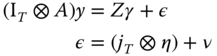
hence it can be estimated by “plugging into” the general likelihood (10.9) the particular scaled error covariance ![]() characterized by one parameter:
characterized by one parameter: ![]() , the ratio of the variance of the individual effect over that of the idiosyncratic error.
, the ratio of the variance of the individual effect over that of the idiosyncratic error.
Error Structures
As already discussed, the spatial error, random effects model gives rise to two possible specifications, depending on the interaction between the spatial autoregressive effect and the individual error components: the ![]() specification first analyzed by Anselin (1988) where only the idiosyncratic error is spatially correlated:
specification first analyzed by Anselin (1988) where only the idiosyncratic error is spatially correlated:
with the scaled errors' covariance (denoting ![]() and
and ![]() ):
):
and that of Kapoor et al. (2007) where the same spatial process applies both to the individual and the idiosyncratic error component:

where the scaled errors' covariance is:
10.3.3.3 Generalized Moments Estimation
The computational intensity of ML estimation, which in the simpler models is related mostly to the need to recompute the determinants at each optimization step, has long been a limiting factor in practical applications. Samples of cross‐sectional size in the hundreds were the practical maximum for the simple SAR or SEM models at the end of the 20th century, both because of the difficulty in obtaining a result at all and of the numerical unreliability of the latter if any because of precision problems (Kelejian and Prucha, 1999, Bell and Bockstael, 2000). Today, much more powerful computers have extended the scope of ML methods, but on the other hand the increasing availability of GIS data has brought forward a new generation of estimation problems of ever increasing size (an early survey and examples in Bell and Bockstael, 2000).
This has prompted researchers to explore alternative estimation strategies. Kelejian and Prucha (1999) proposed the generalized moments (GM) method, which, despite being asymptotically equivalent to ML under normality of the errors, is consistent irrespective of the latter; computationally, moreover, it does not require the numerically cumbersome calculation of the determinants.
The GM estimator for the cross‐sectional SEM model (see also Bell and Bockstael, 2000) is based on the following three moments of the error term:
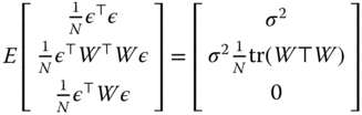
The estimation strategy is based on the idea of estimating the spatial autoregressive coefficient ![]() based on the residuals from a consistent estimator (here, OLS) and then using it in a feasible GLS analysis. With respect to maximum likelihood, the GM estimator has the additional advantage of not relying on a normality assumption for the errors. One drawback is that standard errors are not available for the
based on the residuals from a consistent estimator (here, OLS) and then using it in a feasible GLS analysis. With respect to maximum likelihood, the GM estimator has the additional advantage of not relying on a normality assumption for the errors. One drawback is that standard errors are not available for the ![]() parameter.
parameter.
The Kelejian and Prucha (1999) GM estimator has first been extended to the panel case by Druska and Horrace (2004), then by Kapoor et al. (2007) who estimated the above described ![]() model with RE, a specification which, after them, is known as KKP. In order to perform feasible GLS, one does now need consistent estimates of the spatial autoregressive parameter
model with RE, a specification which, after them, is known as KKP. In order to perform feasible GLS, one does now need consistent estimates of the spatial autoregressive parameter ![]() and the two variance components of the composite error,
and the two variance components of the composite error, ![]() and
and ![]() . The
. The ![]() estimator a la KKP estimates them based on six moment conditions, using the OLS residuals
estimator a la KKP estimates them based on six moment conditions, using the OLS residuals ![]() , which are still consistent in this setting:
, which are still consistent in this setting:

where ![]() ,
, ![]() ,
, ![]() , and
, and ![]() ; and
; and ![]() and
and ![]() are, respectively, a time‐demeaning and a time‐averaging matrix.
are, respectively, a time‐demeaning and a time‐averaging matrix.
The moment conditions are now redundant and can be employed in different ways. The simplest is to consider only the first three moment conditions. The second way is to employ all six moments in estimating the three unknown parameters, weighing them through a covariance matrix calculated under the assumption of normally distributed errors. The third and last proceeds like the second, using all available moments but employs a simplified weighting matrix.
GM methods have been extended to the other relevant specifications in spatial econometrics. Spatial fixed effects models can also be estimated in this framework, through a modification of the KKP procedure suggested by Mutl and Pfaffermayr (2011) and consisting in replacing the OLS residuals, inconsistent under the fixed effects assumption, with spatial 2SLS within residuals; the spatial parameter ![]() is estimated by an adaptation of the simplified KKP procedure (first three moment conditions only) and used in a spatial Cochrane‐Orcutt transformation of the within‐transformed variables. The GM method has also been extended to the SAR and SAREM models, so that now any combination of spatial lag and error, with individual effects of either random or fixed type, can be estimated through this numerically very efficient method (see Millo and Piras, 2012).
is estimated by an adaptation of the simplified KKP procedure (first three moment conditions only) and used in a spatial Cochrane‐Orcutt transformation of the within‐transformed variables. The GM method has also been extended to the SAR and SAREM models, so that now any combination of spatial lag and error, with individual effects of either random or fixed type, can be estimated through this numerically very efficient method (see Millo and Piras, 2012).
10.3.4 Testing
10.3.4.1 LM Tests for Random Effects and Spatial Errors
Requiring only the estimation of the restricted specification, Lagrange multiplier (LM) tests in the tradition of Breusch and Pagan (1980) are particularly appealing in a spatial random effects setting because of the computational difficulties related to ML estimation of encompassing models.
Baltagi et al. (2003b) derived joint, marginal and conditional tests for all combinations of random effects and spatial correlation. Starting from the random effects model with SEM errors (![]() ), the error term can be written as:
), the error term can be written as:
and the (unscaled) variance covariance matrix of the errors as:
The hypotheses under consideration are:
 under the alternative that at least one component is not zero
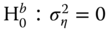 assuming no spatial correlation, under the one‐sided alternative that the variance component is greater than zero
 assuming no random effects, under the two‐sided alternative that the spatial autocorrelation coefficients is different from zero
 assuming the possible existence of random effects, under the two‐sided alternative that the spatial autocorrelation coefficient is different from zero
 assuming the possible existence of spatial autocorrelation and the one‐sided alternative that the variance component is greater than zero
The joint LM test for the first hypothesis of no random effects and no spatial autocorrelation (![]() ) is given by:
) is given by:
where ![]() ,
, ![]() ,
, ![]() and
and ![]() denotes OLS residuals. The marginal LM test for random effects assuming no spatial correlation is given by:
denotes OLS residuals. The marginal LM test for random effects assuming no spatial correlation is given by:

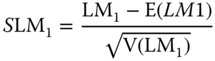
An alternative standardized version with better finite sample properties can be obtained by centering and scaling the one‐sided LM statistic:
Analogously, the marginal LM test of no spatial autocorrelation assuming no random effects is given by:

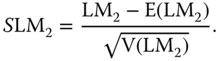
which also admits a standardized form with better properties:
![]() and
and ![]() are asymptotically normally distributed as
are asymptotically normally distributed as ![]() for fixed
for fixed ![]() , under
, under ![]() and
and ![]() respectively. Based on the latter, a one‐sided joint test statistic for
respectively. Based on the latter, a one‐sided joint test statistic for ![]() can be derived as:
can be derived as:
which is asymptotically distributed as a standard normal. In practical applications ![]() can turn out negative, especially when the random effects variance is small, and the same applies to
can turn out negative, especially when the random effects variance is small, and the same applies to ![]() when the spatial autocorrelation coefficient is small. A test for the joint null hypothesis can therefore be based on the following decision rule:
when the spatial autocorrelation coefficient is small. A test for the joint null hypothesis can therefore be based on the following decision rule:

Under the null the test statistic ![]() has a mixed
has a mixed ![]() ‐distribution given by:
‐distribution given by:
When using ![]() , one is assuming that random regional effects do not exist. However, especially when the random effect variance is actually large, this may lead to incorrect inference. For this reason Baltagi et al. (2003b) derived a conditional LM test for spatial autocorrelation allowing for the random effects variance to be non‐zero. The expression for the test assumes the following form:
, one is assuming that random regional effects do not exist. However, especially when the random effect variance is actually large, this may lead to incorrect inference. For this reason Baltagi et al. (2003b) derived a conditional LM test for spatial autocorrelation allowing for the random effects variance to be non‐zero. The expression for the test assumes the following form:

where ![]() . Also,
. Also, ![]() ,
, ![]() and
and ![]() .
.
Contrarily to previous tests that use OLS residuals, the residuals ![]() come from the ML estimation of a one‐way error component model. This last point, on the converse, makes the implementation slightly more complicated. A one‐sided test is simply obtained by taking the square root of 10.22. The resulting test statistics are asymptotically distributed as a standard normal. Similarly, when using
come from the ML estimation of a one‐way error component model. This last point, on the converse, makes the implementation slightly more complicated. A one‐sided test is simply obtained by taking the square root of 10.22. The resulting test statistics are asymptotically distributed as a standard normal. Similarly, when using ![]() , one is assuming no spatial error correlation. This assumption may lead to incorrect inference particularly when it is not the case that
, one is assuming no spatial error correlation. This assumption may lead to incorrect inference particularly when it is not the case that ![]() is close to zero. A conditional LM test allowing for spatial error correlation can be derived as:
is close to zero. A conditional LM test allowing for spatial error correlation can be derived as:

where ![]()
![]()
![]()
![]() and
and ![]() . A one‐sided test can be defined by taking the square root of 10.23 based on ML residuals. The test statistic is again asymptotically normally distributed.
. A one‐sided test can be defined by taking the square root of 10.23 based on ML residuals. The test statistic is again asymptotically normally distributed.
10.3.4.2 Testing for Spatial Lag vs Error
If a researcher has a strong reason to expect a spatial‐data‐ generating process to be of the SAR (or, respectively, SEM) kind, then her only problem is to determine whether said spatial effect is present. Then she can either proceed general to specific, estimating the SAR (SEM) model and assessing the significance of the spatial coefficient, or specific to general, testing from the non‐spatial model toward the spatial alternative. In a ML framework, the optimal LM tests for one effect assuming the other out are called marginal. They are dependent on the above hypothesis and will be inconsistent if it is violated; in case only the “other” effect is actually present, they will usually yield a type I error.
As outlined above, although empirical practice has mostly concentrated on either the SAR or the SEM model, estimation of SAREM models containing both a spatial lag and a spatial error is possible. Therefore, if the researcher does not have a strong prior in favor of either, an empirical strategy can be to start from the most general SAREM specification, together with the appropriate kind of individual heterogeneity, and let the data tell us which of the two spatial processes – if any and if not both – did actually generate the observed sample, by looking at the significance diagnostic for either spatial coefficient.
One drawback of this strategy is its computational demands and lesser stability than estimating the simpler models; another is that it does not allow the inclusion of a full set of spatially lagged regressors, a specification approach that has become increasingly popular in recent years.
Lagrange multiplier tests for SAR (SEM) can be either of the conditional type, allowing for the presence of SEM (SAR) tout court, or of the locally robust type, allowing for a limited deviation from zero of the SEM (SAR) coefficient. The former are optimal under the standard assumptions of the ML framework detailed above, and provided the general SAREM model holds; and they require residuals from the restricted SEM (SAR) model. The second kind have suboptimal statistical properties with respect to the optimal conditional tests, and under the above hypotheses on the data‐generating process, they are not guaranteed to hold if misspecification is “too far away,” i.e., if the SAR (SEM) coefficient is of sizable magnitude (and how far is far, i.e., whether 0.1 or 0.4 is tolerable, is an empirical question); moreover the currently available robust LM tests have been developed in a cross‐sectional framework and do not explicitly incorporate panel features. On the other hand, they are computationally simpler being based on the residuals of the non‐spatial model, and they allow including spatially lagged regressors; hence their remarkable success in applied practice.
Marginal vs Locally Robust LM Tests
The original LM tests for either spatial lag or error (Burridge, 1980; Anselin, 1988) were derived in a cross‐sectional context, as tests for, respectively, ![]() vs
vs ![]() assuming
assuming ![]() (henceforth
(henceforth ![]() ); and
); and ![]() vs
vs ![]() assuming
assuming ![]() (henceforth
(henceforth ![]() ). i.e., both can only be employed assuming that the “other” effect is not present. Otherwise, each test has power against the “wrong” alternative as well; therefore, these procedures are of limited value in the model selection process.
). i.e., both can only be employed assuming that the “other” effect is not present. Otherwise, each test has power against the “wrong” alternative as well; therefore, these procedures are of limited value in the model selection process.
Based on the general local robustness framework of Bera and Yoon (1993), in a cross sectional context, Anselin et al. (1996) derived robust LM statistics for ![]() allowing for
allowing for ![]() (henceforth
(henceforth ![]() ) and, respectively, for
) and, respectively, for ![]() allowing for
allowing for ![]() (henceforth
(henceforth ![]() ). These procedures have since been successfully employed in specification searches to discriminate between SAR and SEM models, as formalized in Florax et al. (2003).
). These procedures have since been successfully employed in specification searches to discriminate between SAR and SEM models, as formalized in Florax et al. (2003).
Marginal Spatial LM Tests
In the context of pooled cross sections, without allowing for any correlation feature across either time or cross section (i.e., setting ![]() and
and ![]() in equation ), any cross‐ sectional test can be straightforwardly applied to the pooled dataset. The LM tests of Anselin et al. (1996) (LM) are simply rewritten for the pooled dataset, stacked by cross section, and drawing on an enlarged version of the weights matrix obtained by replicating the cross‐sectional
in equation ), any cross‐ sectional test can be straightforwardly applied to the pooled dataset. The LM tests of Anselin et al. (1996) (LM) are simply rewritten for the pooled dataset, stacked by cross section, and drawing on an enlarged version of the weights matrix obtained by replicating the cross‐sectional ![]() over the main diagonal so that
over the main diagonal so that ![]() (see Anselin et al., 2008). The pooled
(see Anselin et al., 2008). The pooled ![]() test becomes:
test becomes:
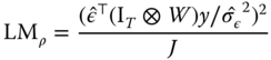
where ![]() are the OLS residuals and
are the OLS residuals and

and
(Elhorst, 2010, Formulae 11 to 13). In turn, the pooled ![]() test is:
test is:
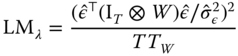
Locally Robust Spatial LM Tests
The robust LM tests of Anselin et al. (1996) can in turn be straightforwardly adapted to the (pooled) panel case, as per Elhorst (2014, Ch. 2.3):
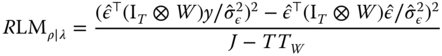
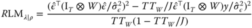
using, again, the OLS residuals ![]() (Elhorst, 2010, Formulae 14‐15).
(Elhorst, 2010, Formulae 14‐15).
Moreover, according to Bera et al. (2009), the LM test for the joint null hypothesis ![]() versus
versus ![]() or
or ![]() is equal to the sum of the marginal test for one effect and the locally robust test for the other:
is equal to the sum of the marginal test for one effect and the locally robust test for the other:
so that the RLM tests can also be obtained indirectly by subtracting the marginal test for the “other” effect from the joint test.
The slmtest function, specifying test = 'lml' ('lme') will perform either the marginal test for SAR (SEM) assuming no SEM (SAR) component in the data‐generating process or the locally robust version if specifying test = 'rlml' ('rlme').
Likelihood‐Based Tests
Given that estimation of the full SAREM model is possible (see the extensive discussion in Millo, 2014), one could directly employ the encompassing model as a specification device, relying on the Wald restriction tests from the general model as an alternative specification strategy instead of looking at the RLM tests. This strategy has the drawback of being computationally more intensive but also some important advantages: the Wald z‐tests for significance of ![]() and
and ![]() are optimal; there is no need for robustification, as the “other” spatial effect is explicitly accounted for in the model, as can be random individual effects; lastly, estimation of the encompassing model also provides the magnitudes of the spatial coefficients together with the significance level of the zero‐restriction tests so that their substantial importance can be assessed.
are optimal; there is no need for robustification, as the “other” spatial effect is explicitly accounted for in the model, as can be random individual effects; lastly, estimation of the encompassing model also provides the magnitudes of the spatial coefficients together with the significance level of the zero‐restriction tests so that their substantial importance can be assessed.
As usual, two kinds of tests are possible from the estimated encompassing model: Wald‐type tests, requiring only an estimate of the latter, and likelihood ratio tests, requiring both the encompassing and the restricted.
Wald Tests
Wald‐type tests are ![]() ‐tests for significance of the relevant parameter in the encompassing model. Thus, from ML estimates of the general SAREM‐RE model,
‐tests for significance of the relevant parameter in the encompassing model. Thus, from ML estimates of the general SAREM‐RE model,
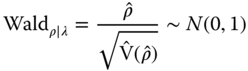
and symmetrically for ![]() . Importantly, the test can be made conditional to (i.e., valid in the presence of) individual random effects by including them in the specification. As observed, fixed individual effects can be eliminated through data transformation in two ways, both familiar from the spatial panel literature: either through time‐demeaning (within transformation) (Elhorst, 2003) or by forward orthogonal deviations (Lee and Yu, 2010a). The former induces residual serial correlation, which can nevertheless be considered (i.e., estimated out) in the encompassing model; while the latter preserves the features of the original errors covariance matrix (Debarsy and Ertur, 2010, p. 7).
. Importantly, the test can be made conditional to (i.e., valid in the presence of) individual random effects by including them in the specification. As observed, fixed individual effects can be eliminated through data transformation in two ways, both familiar from the spatial panel literature: either through time‐demeaning (within transformation) (Elhorst, 2003) or by forward orthogonal deviations (Lee and Yu, 2010a). The former induces residual serial correlation, which can nevertheless be considered (i.e., estimated out) in the encompassing model; while the latter preserves the features of the original errors covariance matrix (Debarsy and Ertur, 2010, p. 7).
LR Tests
Likelihood ratio tests are based on the likelihoods from the general and the restricted model. The test statistic is a simple transform of the difference in likelihoods:
where ![]() is the full vector of ML parameter estimates from the unrestricted model and
is the full vector of ML parameter estimates from the unrestricted model and ![]() from the restricted one, and
from the restricted one, and ![]() the number of restrictions. Thus,
the number of restrictions. Thus,
and symmetrically for ![]() . Again, including random effects in the estimated models makes the test conditional to these effects, while fixed effects can be transformed out as detailed in the previous paragraph but always keeping in mind the effects of the transformation on the error properties.
. Again, including random effects in the estimated models makes the test conditional to these effects, while fixed effects can be transformed out as detailed in the previous paragraph but always keeping in mind the effects of the transformation on the error properties.
10.4 Serial and Spatial Correlation
It is possible to generalize the structure of the errors further by introducing serial correlation in the remainder of the error term, together with spatial correlation and random effects. Baltagi et al. (2007) do so in the context of the Anselin ![]() , specifying the model errors as the sum of an individual, time‐invariant component and an idiosyncratic one that is spatially autocorrelated, as above, but also has serial correlation in the remainder:
, specifying the model errors as the sum of an individual, time‐invariant component and an idiosyncratic one that is spatially autocorrelated, as above, but also has serial correlation in the remainder:

where ![]() is i.i.d.. The combination of this more general error structure, termed
is i.i.d.. The combination of this more general error structure, termed ![]() because of the addition of Serially autoRegressive errors, with a spatially lagged dependent variable and the estimation of the most general model
because of the addition of Serially autoRegressive errors, with a spatially lagged dependent variable and the estimation of the most general model ![]() can still be dealt with in the general ML framework outlined above.
can still be dealt with in the general ML framework outlined above.
10.4.1 Maximum Likelihood Estimation
The model combining spatial and serial correlation with individual effects can be estimated by maximum likelihood, through an extension of the framework outlined in the previous sections of this chapter.
10.4.1.1 Serial and Spatial Correlation in the Random Effects Model
Generalizing the structure of the errors further by introducing serial correlation in the remainder of the error term, together with spatial correlation and random effects, Baltagi et al. (2007) derived a number of conditional and marginal LM tests for the different effects, possibly allowing for the presence of the other ones. Based on their work, Millo (2014) extended the model to include a SAR term. The errors of the SAREM model are specified as in the previous paragraph, so that the full model is:
To derive the likelihood, Baltagi et al. (2007) suggest a Prais‐Winsten transformation of the model with random effects and spatial autocorrelation. Following their simplifying notation, define: ![]() with:
with:

then the expression for the scaled error covariance matrix ![]() can be written as
can be written as
While in principle the inverse and determinant of ![]() can be calculated by brute force, in practice it is convenient, and often necessary, to rely on simplified analytical expressions to reduce the computational burden and extend the range of feasible sample sizes. Baltagi et al. (2007) derived expressions for the inverse and determinant of the error covariance matrix:
can be calculated by brute force, in practice it is convenient, and often necessary, to rely on simplified analytical expressions to reduce the computational burden and extend the range of feasible sample sizes. Baltagi et al. (2007) derived expressions for the inverse and determinant of the error covariance matrix:
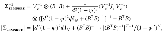
where ![]() and
and ![]() . They can be plugged in the general likelihood (10.9) to estimate the
. They can be plugged in the general likelihood (10.9) to estimate the ![]() model.
model.
10.4.1.2 Serial and Spatial Correlation with KKP‐Type Effects
As an alternative to the ![]() specification, Millo (2014) presents an extension of the
specification, Millo (2014) presents an extension of the ![]() errors a la Kapoor et al. (2007) to serial correlation in the remainder errors. As in the
errors a la Kapoor et al. (2007) to serial correlation in the remainder errors. As in the ![]() case, the random effects are spatially lagged together with the idiosyncratic ones, while the remainder errors
case, the random effects are spatially lagged together with the idiosyncratic ones, while the remainder errors ![]() in turn are serially correlated:
in turn are serially correlated:

This alternative specification assumes that individual effects follow the same spatial diffusion process as the idiosyncratic errors do. By analogy, it is termed ![]() . Just as in the
. Just as in the ![]() case, the error covariance is then again of the
case, the error covariance is then again of the ![]() form (see Section 10.3.3.1), which simplifies computations considerably. In fact, the (scaled) error covariance for this model is:
form (see Section 10.3.3.1), which simplifies computations considerably. In fact, the (scaled) error covariance for this model is:
and, by the properties of Kronecker products, its inverse is
so that there is no need for the numerically demanding and unstable inversion of ![]() .14
.14
10.4.2 Testing
Testing for either effect in the context of the spatially and serially correlated model with individual heterogeneity is performed within the same maximum likelihood framework used for estimation.
10.4.2.1 Tests for Random Effects, Spatial, and Serial Error Correlation
Baltagi et al. (2007) derive the joint, marginal, and conditional LM tests for the model with serial correlation.
They consider all possible combinations of joint, marginal and conditional tests:
- the joint test for
 , (J)
, (J) - the marginal tests for
 and
and  assuming in turn that the other two are zero (M.1‐3)
 - the joint tests for any combination of two of the parameters assuming the third one is zero (M.4‐6)
- the marginal tests for
 and
and  assuming in turn that the other two may or may not be zero (C.1‐3)
 - the joint tests for any combination of two of the parameters assuming the third one may or may not be zero (C.4‐6)
M.1‐3 are well‐established testing procedures in the literature (as observed in Baltagi et al., 2007). M.1 (test for ![]() ) is the LM test for spatial error correlation derived by Anselin (1988) in the context of a pooled model with no serial correlation or individual effects. On the other hand, M.2 (test for
) is the LM test for spatial error correlation derived by Anselin (1988) in the context of a pooled model with no serial correlation or individual effects. On the other hand, M.2 (test for ![]() ) is analogous, for large
) is analogous, for large ![]() , to the well‐known Breusch (1978), Godfrey (1978) serial correlation test. Finally, M.3 is simply the Breusch and Pagan (1980) random effects test.
, to the well‐known Breusch (1978), Godfrey (1978) serial correlation test. Finally, M.3 is simply the Breusch and Pagan (1980) random effects test.
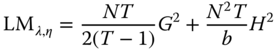
Baltagi et al. (2007, Appendix A.3) show that the test statistic for the joint hypothesis M.4 (![]() ) assuming no random effects is simply the sum of the marginal tests M.1 (
) assuming no random effects is simply the sum of the marginal tests M.1 (![]() ) and M.2 (
) and M.2 (![]() ). Additionally, M.5 is the Baltagi et al. joint test outlined in section 10.3.4.1; and M.6 is the joint test for random individual effects and serial correlation derived in Baltagi and Li (1995) (see section 4.3.2).
). Additionally, M.5 is the Baltagi et al. joint test outlined in section 10.3.4.1; and M.6 is the joint test for random individual effects and serial correlation derived in Baltagi and Li (1995) (see section 4.3.2).
As a result of the previous discussion, we only consider the three‐way joint test J and the one‐way conditional tests C.1‐3.
The corresponding null hypotheses are:
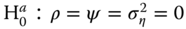 under the alternative that at least one component is not zero (J)
 , assuming
 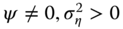 : test for spatial correlation, allowing for serial correlation and random individual effects (C.1)
 , assuming
  : test for serial correlation, allowing for spatial correlation and random individual effects (C.2)
 , assuming
  : test for random individual effects, allowing for spatial and serial correlation (C.3)
The joint LM test for ![]() is given by:
is given by:
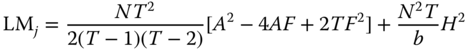
where, ![]() ,
, ![]() ,
, ![]() ,
, ![]() ,
, ![]() is a matrix with bidiagonal elements equal to one and
is a matrix with bidiagonal elements equal to one and ![]() denotes OLS residuals. Under
denotes OLS residuals. Under ![]() ,
, ![]() is distributed as
is distributed as ![]() .
.
The conditional C.1 test for ![]() gives rise to the following statistic, asymptotically distributed as
gives rise to the following statistic, asymptotically distributed as ![]() under
under ![]() :
:

where
is the score vector (evaluated at the null), ![]() a vector of ML residuals obtained from the estimation of the model with individual error components and serial correlation,
a vector of ML residuals obtained from the estimation of the model with individual error components and serial correlation, ![]() , and
, and ![]() has been defined above.
has been defined above.
The conditional C.2 test for ![]() is based on the following statistic, asymptotically distributed as
is based on the following statistic, asymptotically distributed as ![]() under the null:
under the null:
where ![]() is the corresponding element of the information matrix,15
is the corresponding element of the information matrix,15
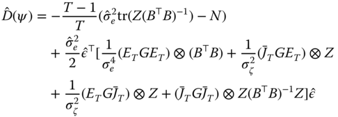
with ![]() the score evaluated at the null and
the score evaluated at the null and ![]() the vector of ML residuals from the estimation of a panel model with individual error components and serial correlation. Both
the vector of ML residuals from the estimation of a panel model with individual error components and serial correlation. Both ![]() and
and ![]() assume the same expression as before, while as usual
assume the same expression as before, while as usual ![]() .
.
The conditional C.3 test for ![]() is based on the following statistic:
is based on the following statistic:
where

is the score evaluated at the null, ![]() is the corresponding element of the information matrix16 and
is the corresponding element of the information matrix16 and ![]() is the vector of estimated residuals from the ML estimation of a panel model with spatially and serially correlated errors but no individual error components. The
is the vector of estimated residuals from the ML estimation of a panel model with spatially and serially correlated errors but no individual error components. The ![]() test statistic is asymptotically distributed as
test statistic is asymptotically distributed as ![]() under
under ![]() :
:
10.4.2.2 Spatial Lag vs Error in the Serially Correlated Model
Testing for spatial lag vs spatial error in a model allowing for random effects and/or serially correlated errors can be done via the Wald approach, from the encompassing specification.17