7.7. Discrete State Equations of Boost and Buck Converters
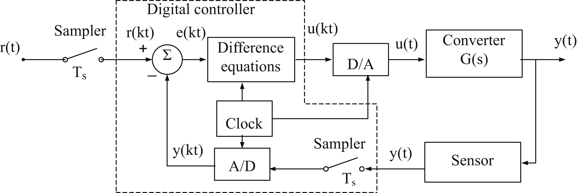
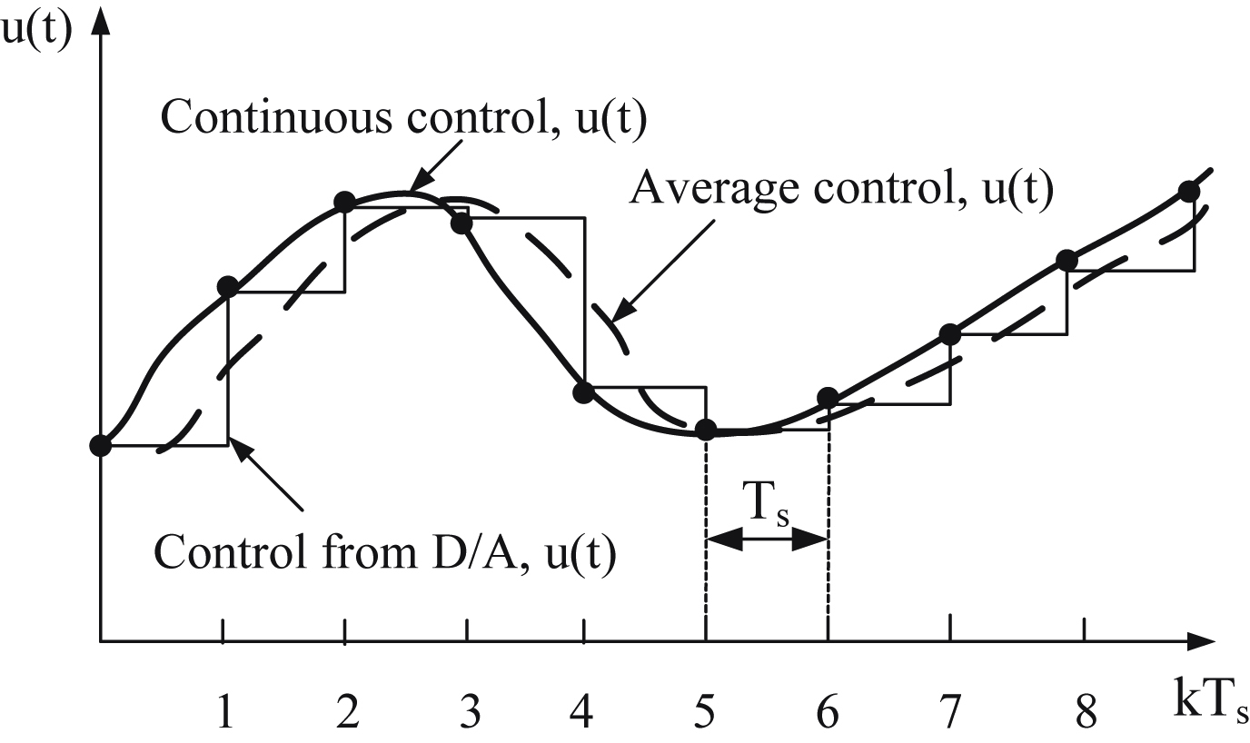
Fig. 7.26 presents the block diagram of the digital controller of a dc–dc converter. Moreover, Fig. 2.27 presents the control signal u(t) in continuous control, average control, and control from D/A.
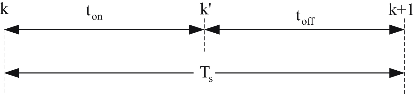
Suppose that an operation cycle of a boost converter lasts from the time instant kTs to (k+1)Ts as shown in Fig. 7.28.
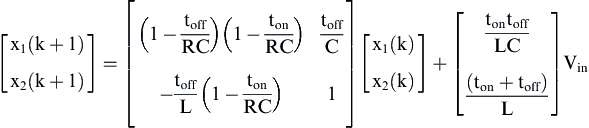
Assuming that the switching period Ts is too small, the following approximate discrete time model holds:
x→(k+1)−x→(k′)toff=A1x→(k′)+BVin
(7.125)
or
x→(k+1)=(I+toffA1)x→(k′)+BtoffVin
(7.126)
where I=2×2 unit matrix.
Figure 7.26 Block diagram of the digital controller of a dc–dc converter.
Figure 7.27 Different types of control signals.
Figure 7.28 One operational discrete cycle of the boost converter.
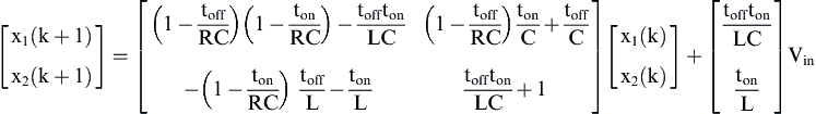
These equations are valid from the instant time kTs to k′Ts. Since the switching period Ts is too small, the following discrete time model is applied:

 (7.130)
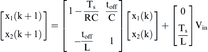 (7.131)
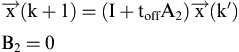 (7.135)
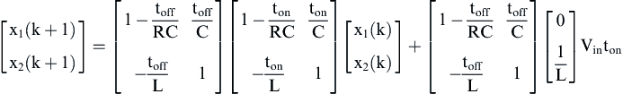
 (7.137)
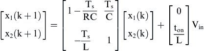 (7.138)