
12.5. Synchronous Motor Drive Systems
12.5.1. Permanent Magnet (PM) Synchronous Motors
PM synchronous motors are constantly gaining popularity among the scientific community, especially in the fields of electric traction and power generation. This occurs mainly due to their inherent advantages of high power density, high efficiency, and reliability. Their performance and efficiency have rendered them the dominant choice in many applications. Permanent magnet motor (PMM) is related to the classical synchronous motor with the difference that the dc winding is replaced by PMs that produce steady magnetic flux. This way the copper losses in the rotor are eliminated, since there is no field winding and, consequently, the overall motor efficiency is increased. Additionally, the high efficiency values incur significant reduction in the motor size and weight (high power density) and lower moment of inertia. On the other hand, however, the control systems are very complicated due to the permanent nature of the excitation that can cause rotor demagnetization phenomena.
12.5.1.1. PM Motor Rotor Configurations
PMMs can be classified, based on the rotor configuration that occurs, into the following:
1) Surface-mounted PM motors with sinusoidal flux
In this type of PMM, the stator comprises a sinusoidal three-phase winding, which produces an air-gap flux rotating with the synchronous speed. The PMs are placed on the rotor surface using epoxy glue. The rotor magnetic circuit is either made of compact or laminated steel. In the case of variable speed operation, the motor can include a squirrel-cage or a damping winding, which of course incurs additional ohmic losses. If the machine operates as a generator, rotated by an external source, then the stator windings produce symmetrical sinusoidal three-phase voltages. Since the magnets magnetic permeability is very close to that of the air (μr ≈ 1) and the magnets are placed on the rotor surface, the machine active air-gap length is very big and it exhibits practically no saliency. This contributes to the limitation of the armature reaction phenomenon due to the low values of magnetizing inductance.
2) Interior PM motors with sinusoidal flux
Contrary to surface-mounted PMMs, in an interior PMM the magnets are placed inside the rotor body. Several different geometric configurations of rotor structures with interior magnets have been tested and reported in recent bibliography, mainly regarding the magnet shape and orientation. The stator comprises a conventional three-phase sinusoidal winding. The main characteristics of interior PMMs are the following:
• The motor structure is very compact and mechanically robust, allowing higher operating speed values
• The motor active length is small, which incurs higher armature reaction
• The motor active length is higher along the d axis than along the q axis, therefore the motor exhibits high saliency
3) Surface-mounted PM motors with trapezoidal flux
A synchronous PMM with trapezoidal flux is a motor that exhibits no saliency, like a sinusoidal flux surface-mounted PMM, but comprises a stator with concentrated windings instead of sinusoidal distributed windings. To increase the sinusoidality of the produced magnetic field distribution in trapezoidal flux motors the use of fractional slot windings is a common practice. As the motor rotates, the magnetic flux that is associated with a specific phase winding varies linearly with time, except for the instant that the gap between the magnets aligns with the phase axis. If the motor is rotated by an external mechanical source, which means that operates as a generator, the phase voltages will exhibit symmetrical trapezoidal waveforms. For this reason, the use of an electronic converter is necessary, to produce six step current waveforms in the motor terminals, to be able to produce mean electromagnetic torque. Since the use of the converter is mandatory, this type of motors is utilized as electronic motors. Through the use of an inverter and an absolute position sensor that is placed on the motor shaft, trapezoidal flux motors can be controlled and operated as brushless dc motors. Trapezoidal flux motors have more similar performance characteristics to the dc motors than the sinusoidal flux motors. They are simple, less expensive and have higher torque density values than sinusoidal motors. They are typically used in low-power drive systems, as servomotors and in domestic applications where the phenomena associated with brushed dc motors have to be avoided.
12.5.1.2. Mathematical Model of PM Motors
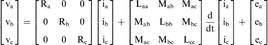
For the analysis and the control of the synchronous PMM two models have been reported. The abc coordinates model and the dynamic d–q model. The first is preferred for the analysis of problems involving harmonic components, and the second is used for the transient analysis of the motor operation. The majority of the control strategies of PMMs are based on the dynamic d–q model. Fig. 12.56 shows the equivalent circuit of a synchronous PMM according to the abc coordinates model.
The voltage equations of synchronous PMM are:
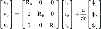 (12.161)
where Ra is the resistance of the phase a, ia is the current of the phase a, and ψa is the magnetic flux of the phase a.
The magnetic flux equations can be derived as:
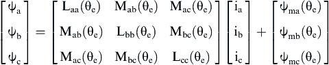 (12.162)
where Laa is the self-inductance of the a-phase winding, Mab is the mutual inductance between the windings of the a and b phases, and ψma is the remanence flux due to the PMs in the phase a.
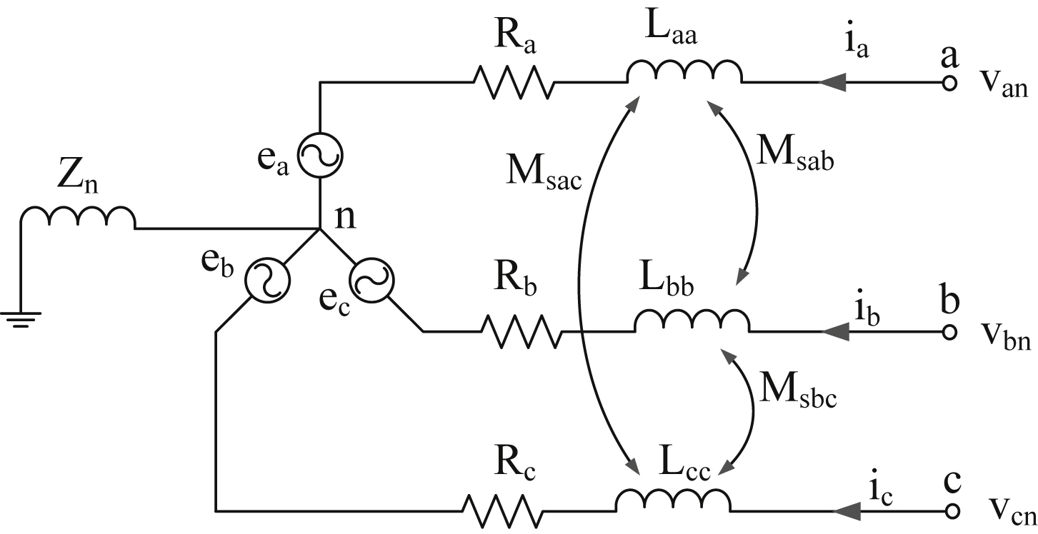
Figure 12.56 Equivalent circuit of a synchronous permanent magnet motor according to the abc coordinates model.
Due the magnetic saturation and the mechanical construction of the synchronous PMM, the self and mutual inductances are functions of the electrical angle of the rotor θr, which is equal to the synchronous angle θe. The electrical angle of the rotor is practically the direction of rotor magnetic flux (north pole of the rotor magnets). At zero angle, the flux direction aligns with phase a. The relation between the mechanical and the electric rotor angle is given:
![]() (12.163)
(12.163)
In the general case, the inductances of a synchronous PMM consist of a constant component and a sum of odd harmonics associated with the variation of the electrical rotor angle. As far as the control of ac motors, according to modern bibliography, the following assumptions are made:
• The stator windings are considered sinusoidally distributed and the effect of the specific geometry of the stator teeth is neglected. The magnetomotive force produced by the stator is considered sinusoidal.
• The radial distribution of the magnetic flux density produced by the PMs is considered sinusoidal.
• The magnetic flux associated with the stator armature reaction only involves the fundamental component.
• The magnetic saturation is neglected.
Considering the above mentioned assumptions, the variations of the inductances contain only a sinusoidal component, and since the inductance of each phase is maximum when the magnetic flux is aligned with the phase, can be concluded (see Eq. 12.164 for θe = 0) that the values of the inductances are functions of the angle 2θe. If also a sinusoidal distribution of the saliency is considered, the mutual and self inductances of the windings can be written as follows:
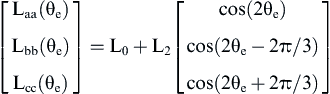 (12.164)
and
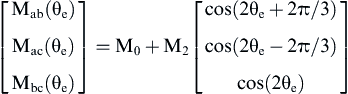 (12.165)
where L0 and M0 are the mean components of the self and mutual inductances, respectively, L2 and M2 are the respective amplitudes of the sinusoidal components. Finally, the flux produced by the PMs is a function of the rotor electrical angle and can be written as:
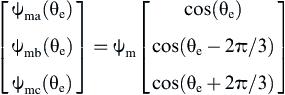 (12.166)
Under no load operation, the equations for the induced EMF by the PM excitation are obtained:
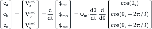
or
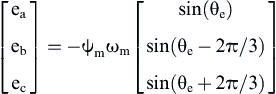 (12.167)
where ωm is the mechanical synchronous rotating speed.
 (12.168)
The produced electromagnetic torque is given:
![]() (12.169)
(12.169)
12.5.1.2.1. Dynamic d–q Model of Permanent Magnet Motors
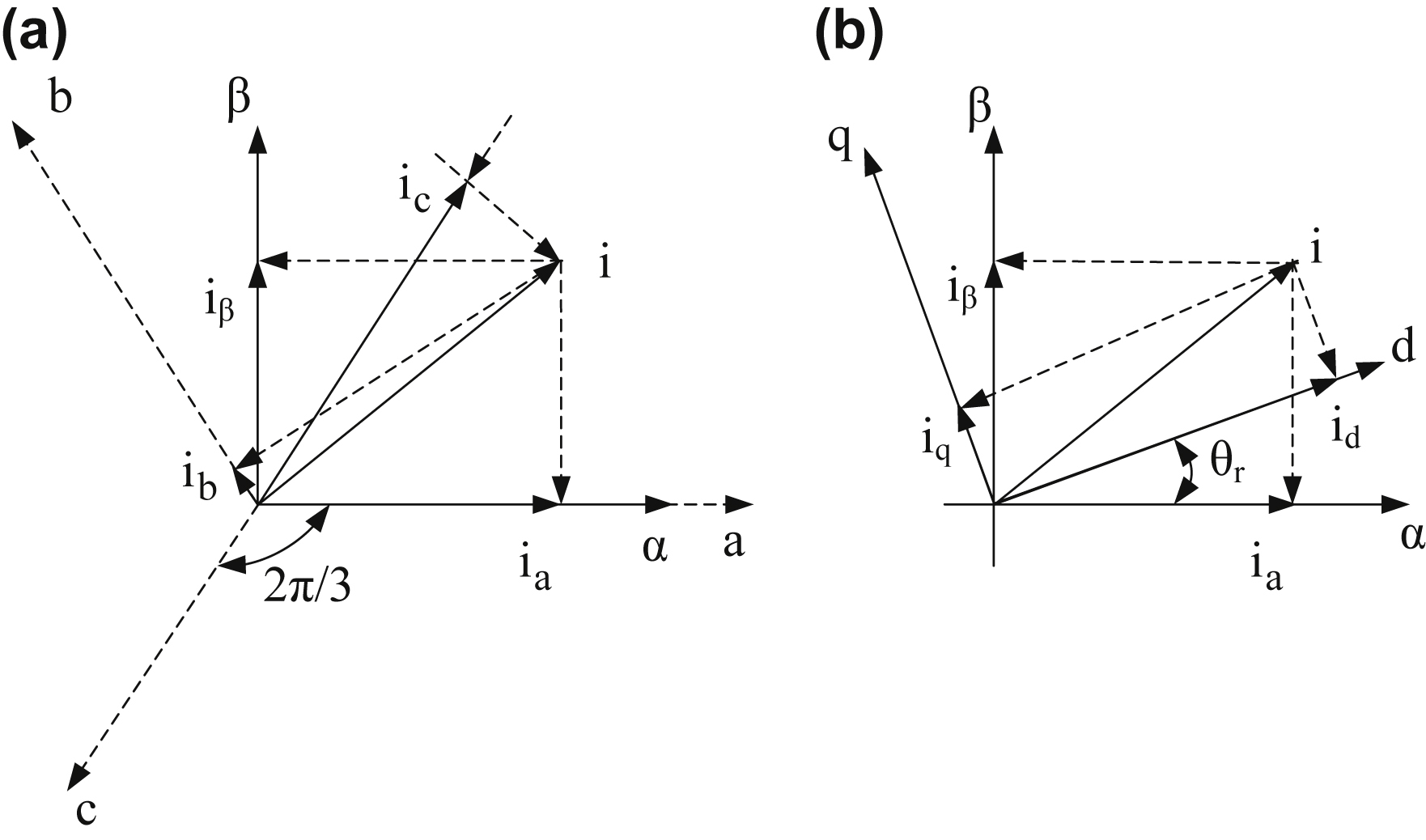
The per-phase equivalent circuit developed in the previous paragraph becomes very complicated when associated with a rotating system where the phase inductances of the stator and the respective mutual inductances are functions of the rotor electrical angle. Therefore, for the analysis of a VSD system a model that does not include the time-varying inductances, which occur due to the relevant movement between the electrical circuits, has to be developed. For the analysis of ac systems the approach of three-phase components through the use of complex phasors has been adopted. These phasors are called space vectors and will be explained later.
Any three-phase variable x can be represented by a complex phasor (space vector) through the Clarke transformation. Variable x, that can be either the magnetic flux or the phase current or the phase voltage, is multiplied by the matrix K of the transformation to be transformed into a space vector xα + j xβ:
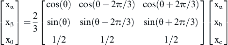 (12.170)
For the inverse transformation, the inverse matrix is utilized:
 (12.171)
In Eq. (12.171) the angle θ represents the angle between the real axis of the complex plane and the direction of phase a. This angle can be chosen at will. The coefficient 2/3 in the equation of the transformation refers to the use of the simple coordinate transformation where the length of the space vector xa + j xβ is equal to the peak value of the three-phase variable x. Finally, the zero-order component x0 has nonzero values only in case of faults (i.e., phase asymmetries). For the rest of the analysis, the zero-order component will be neglected. For the control of synchronous PMMs the typical choices for the value of the angle of the reference frame is 0 and the rotor electrical angle θe. If the angle is zero the transformation is associated with the stator reference frame, where the real axis is aligned with phase a. Since the angle value is maintained at 0, the reference frame is called stationary reference frame and the transformation is known as Clarke transformation. If the reference frame angle is chosen to be θe, then the real axis of the complex plane is rotated synchronously to the motor rotor. In that case, the synchronous (rotor) reference frame is considered. Bibliographically, Park transformation refers to the transformation to the rotating reference frame, while Clarke transformation refers to the stationary reference frame (Fig. 12.57).
Through the use of the Park transformation, the mathematical model of the synchronous PMM is significantly simplified. In the rotating d–q reference frame, the voltage equations are:
![]() (12.172)
(12.172)
![]() (12.173)
(12.173)
The d-axis and q-axis flux components are obtained, for the rotating reference frame:
![]() (12.174)
(12.174)
![]()
![]() (12.175)
(12.175)
where
![]() (12.176)
(12.176)
![]() (12.177)
(12.177)
Substituting Eqs. (12.174) and (12.175) into (12.172) and (12.173) the voltage equations can be rewritten:
![]() (12.178)
(12.178)
![]() (12.179)
(12.179)
The electromagnetic torque in the rotating reference frame is also obtained:
![]() (12.180)
(12.180)
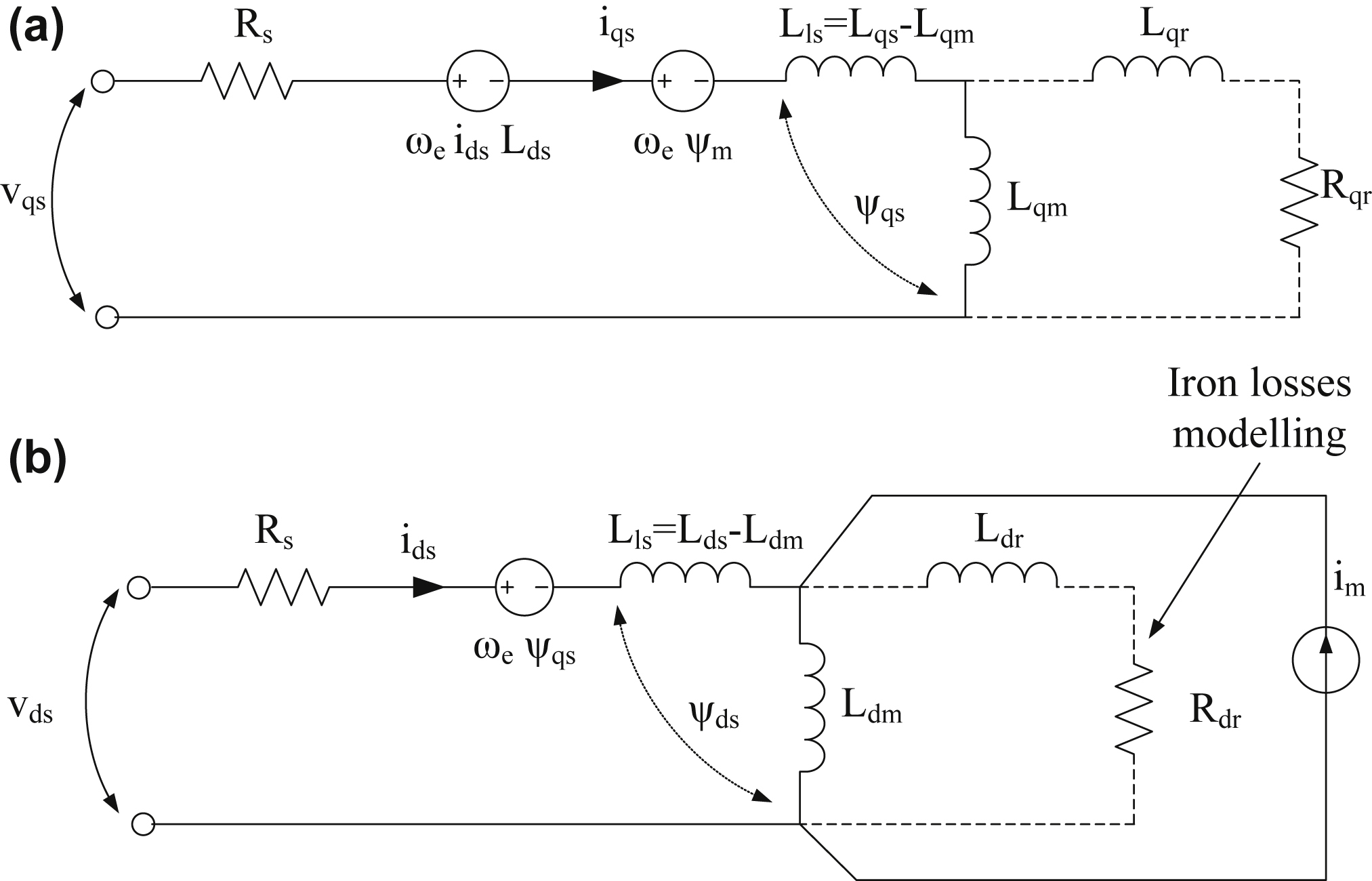
The equivalent circuits of the q- and d-axis for the synchronously rotating reference frame of the PMM is shown in Fig. 12.58.
It is worth mentioning that the d–q analysis model is valid for both surface-mounted and interior PMM with sinusoidal flux, but not for trapezoidal flux motors. The difference between the surface-mounted and interior PMMs lies in the different saliency values that incur different values for the d-axis and q-axis inductances for the interior PMM.
12.5.1.3. PM Motor Control Techniques
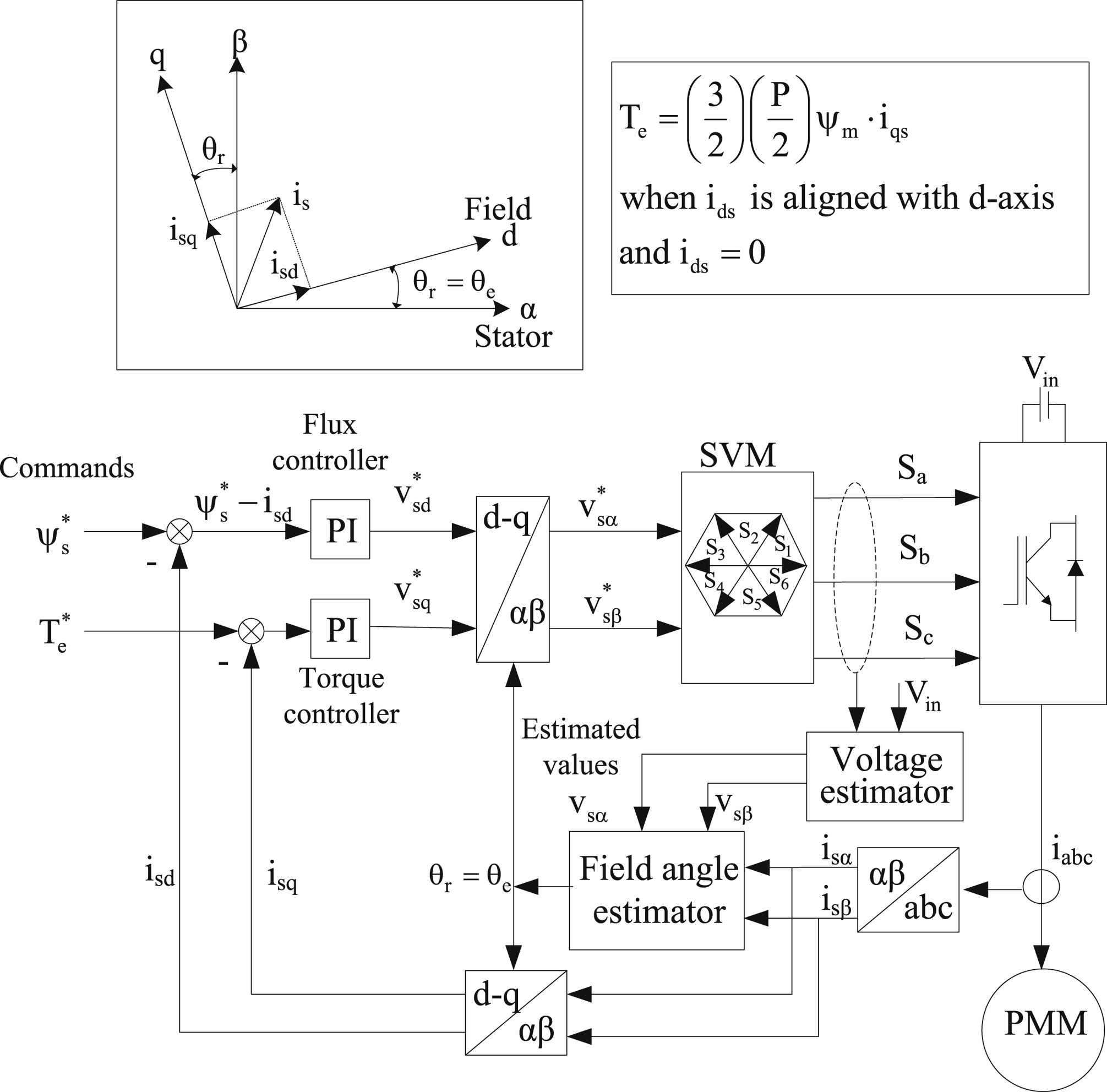
The general block diagram of the control strategy of a high-efficiency PMM is shown in Fig. 12.59. The core of the system consists of the internal flux control loop, the internal torque control loop, and the estimator, which can be implemented with various different ways. The external speed control loop is practically the same for every control technique and produces flux and torque commands using the appropriate controllers. The speed feedback signal can be acquired through a mechanical movement sensor (i.e., encoder or resolver) or can be estimated providing the capability for sensorless control.
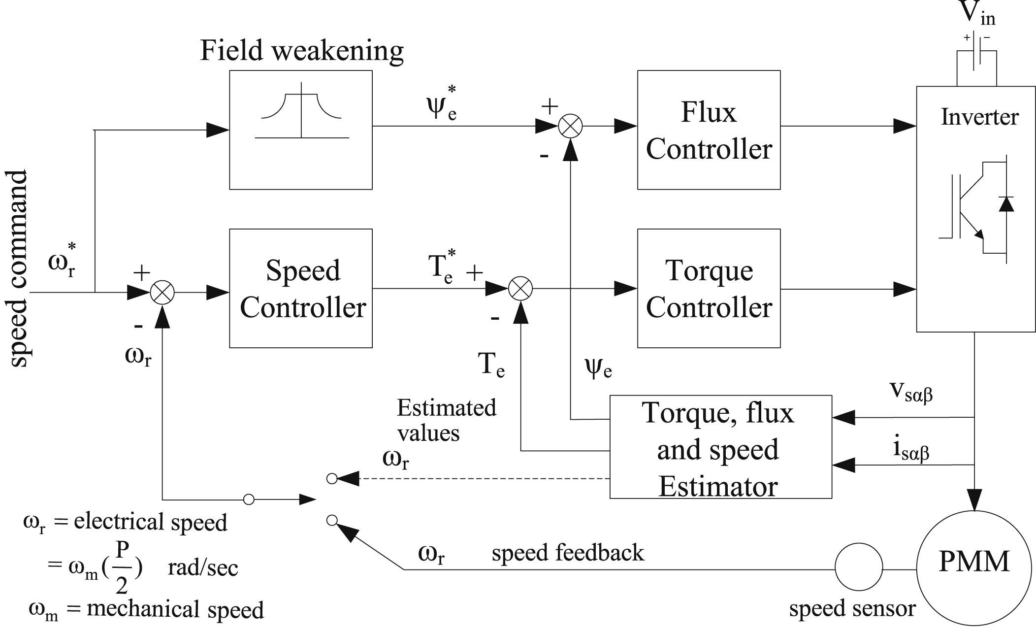
Figure 12.59 Block diagram of the flux controller of a permanent magnet motor comprising internal flux and torque control loops.
12.5.1.3.1. Scalar V/f Open Loop Control
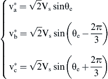
Scalar control only alters the amplitude of the control variables and neglects the coupling of the motor's equations. Therefore, both the voltage of the motor and the frequency of its phase currents simultaneously affect and control both the magnetic flux and the electromagnetic torque of the motor. As a result, the coupled nature of the motor's equations prevents the achievement of high performance levels. However, drive systems with scalar controllers are currently very popular in low power applications with relatively low construction cost. Fig. 12.60 shows the block diagram of the scalar V/f speed control methodology, which is the most popular open loop control methodology with independent frequency control.
Scalar control is based on the demand for constant stator magnetic flux, to maximize the produced electromagnetic torque. To maintain a constant flux value, the ratio of the motor voltage to the motor frequency should remain constant (V/f = const). For this reason, the phase voltage–amplitude command  is produced by the frequency control command through the gain factor G. For low-speed operation, the voltage drop along the stator winding is significant and, consequently, the produced magnetic flux is limited. To avoid this phenomenon and to maintain the value of the magnetic flux near the nominal for low-speed operation, a boost voltage Vo is added to the reference amplitude of the phase voltage. The impact of the boost voltage is negligible in higher frequencies.
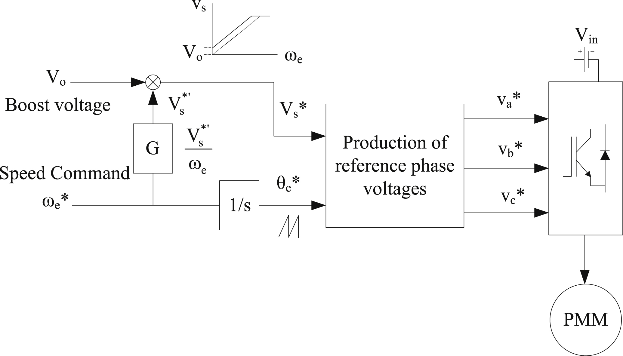
Finally, the reference speed signal  is integrated, producing the reference angle signal
  and the respective reference phase voltages
  ,
,  , and
, and  are produced as:
 (12.181)
It should be noted, that the PWM controller is integrated in the inverter block. In Fig. 12.61 the operation regions of the control system are shown. Both motor and generator operation mode are considered. Considering zero initial load torque TL on the motor axis, the motor can easily start rotating and go from operating point 0 to operating point A, slowly increasing its frequency. At this point, the load torque starts to gradually increase. In steady-state operation, where TL = Te, the operating point will move vertically along AB in the first quadrant. The electromagnetic torque is given by:
![]() (12.182)
(12.182)
where
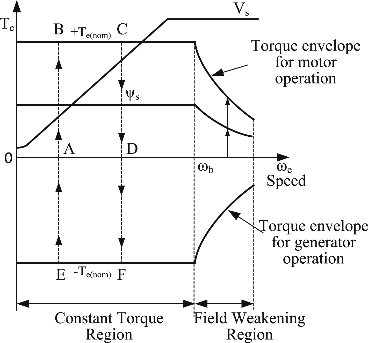
Therefore, for a constant value of the stator magnetic flux ψs, the power angle and the stator current will gradually increase until the production of the nominal value of electromagnetic torque at point B. At that point, either the power angle has reached its boundary value (π/2) or the stator current has reached its nominal value. Usually, the operation of the system reaches the current limit of the inverter before the stability limit of the motor δ = π/2. The operating point can change from B to C by gradually increasing the frequency command. Finally, the system can return to operating point D by gradually reducing the load torque.
At nominal speed (ωb), the voltage will saturate. Beyond that point, the motor enters the flux weakening operating region. That way, the maximum available torque is reduced due to the reduced stator magnetic flux ψs, as shown in Fig. 12.61. Any rapid change in the signal can lead to system instability due to loss of synchronization. For variable speed operation, the speed of the motor should follow the frequency command without losing synchronization. The rate of change of the signal or the maximum acceleration/deceleration capability is dictated by the following equation:
![]() (12.183)
(12.183)
where J is the moment of inertia,  is the synchronous rotational speed, P is the number of poles, and ωm is the mechanical speed in rad/s. Consequently, the maximum acceleration and deceleration capability are respectively given by:
![]() (12.184)
(12.184)
![]() (12.185)
(12.185)
where the nominal electromagnetic torque Te(nom) and the load torque TL contribute to the deceleration of the motor.
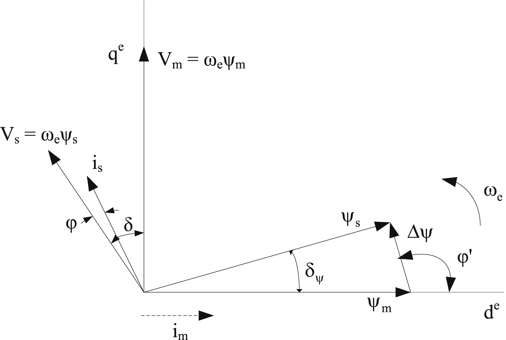
At point A, if the speed command is a ramp function with high slew rate, the produced electromagnetic torque will jump to point B and the motor will accelerate along the segment BC until the speed reaches a steady state at point D. Similarly, the operating point sequence for deceleration is D-E-F-A. The electric energy that is gained during deceleration can be consumed in a dynamic brake or can be induced back to power source (i.e., in case it is composed of batteries). The rotation of the motor towards the opposite direction can be achieved through the inversion of the sequence of two phases of the inverter. In Fig. 12.62 the vector diagram of the PMM is given. The stator resistance is considered negligible and the magnetic flux of the rotor excitation ψf is chosen as the reference vector. The vector of the constant equivalent excitation current If for a PMM is also shown.
12.5.1.3.2. Linear Torque Control Methods
Over the last 40 years, various closed loop torque control techniques has been developed. However, not all have been successfully introduced to industrial applications. In this section the most popular and widely used control strategies along with some new and promising ones will be introduced. The control strategies can be classified into two main categories: linear and nonlinear. Linear torque controllers operate combined with PWM techniques. They initially calculate the mean required voltage vector in a period. The vector is composed through a PWM technique, which in most cases is the SVM technique. Contrary to nonlinear control techniques, linear torque control (TC) methodologies employ linear PI (proportional-integral) controllers. The sampling frequency ranges from 2 to 5 kHz, while for nonlinear controller it reaches a value of 40 kHz. In the following paragraphs most important linear control techniques will be analyzed, namely, the FOC, DTC-SVM, and the direct torque control with flux space vector modulation (DTC-FVM).
12.5.1.3.3. Field-Oriented Control (FOC)
FOC was proposed during the 1970s from Hasse and Blaschke and is based on the analogy of the ac motor with the dc motor, where the current commutation is achieved mechanically. In the dc motor the magnetic flux is separately controlled by the excitation current, while the torque is controlled by the armature current. Therefore, the two currents are electrically and magnetically decoupled. On the contrary, in AC motors, the armature current of the stator affects both the magnetic field and the produced torque. The decoupling of flux and torque can be achieved using the analysis of the instantaneous current into two components: the field current and the current associated with the development of torque, in a rotor reference rotating frame, as shown in Fig. 12.63. This technique enables the control of the motor in a way very similar to the control of a dc motor with independent excitation and can be implemented through current control with linear PI controller and a PWM inverter using an SVM technique. The core of this control system consists of the reference frame transformation blocks, that render the calculation of the d-axis and q-axis currents (isd and isq) and the reference voltage vectors (vsα∗ and vsβ∗) feasible, through the αβ/dq and dq/αβ transformation, respectively. Therefore, this control scheme allows for indirect control of the developed torque and magnetic field through current vectors aligned with the rotor magnetic field.
12.5.1.3.4. Direct Torque Control With Space Vector Modulation (DTC-SVM)
Direct torque control can be considered a simplified version of the FOC oriented to the stator field and without any current control loops. Its operation is based on the equation of the developed electromagnetic torque of the motor. According to it, the developed torque is proportional to the amplitude of the PM flux vector, the amplitude of the stator flux vector, and the angle between them. Therefore, the maintenance of the amplitude of the stator flux vector at a constant value, allows for precise control of the electromagnetic torque through the variation of the angle of the two flux vectors. By neglecting the variation of the stator resistance, the variation of the stator flux is proportional to the applied voltage. Consequently, the developed torque can be controlled by rapidly changing the flux direction through the control of the applied voltage.
The block diagram of the DTC-SVM scheme with closed loop torque and flux control is shown in Fig. 12.64. The output signals of the PI controllers are the reference stator voltage signals vψ∗ and vT∗, oriented towards the stator magnetic field (dq). These dc command signals are transformed into stationary coordinates (αβ) and the command signals vsα∗ and vsβ∗ are applied into the SVM block. It should be noted, that the specific control scheme is very similar to the classic switching table DTC (ST-DTC) scheme, which is shown in Fig. 12.65, where the switching table has been replaced by an SVM block and the flux and torque hysteresis controllers have been replaced by PI controllers. In the DTC-SVM scheme, the torque and flux are directly controlled through closed loop and, consequently, a precise torque and field estimation is mandatory.
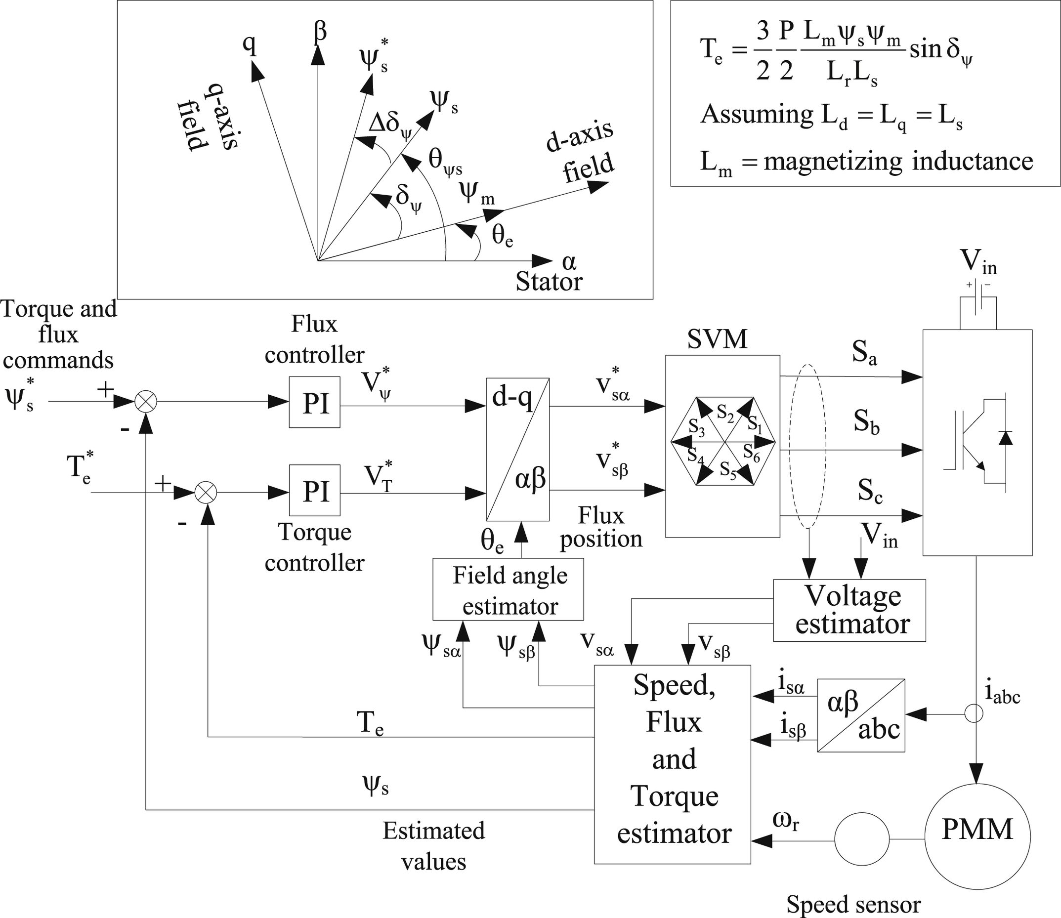
This specific control technique, unlike the ST-DTC operates with a constant switching frequency. This feature improves the performance of the overall system, as it reduces the flux and torque fluctuations and offers improved low-speed operation.
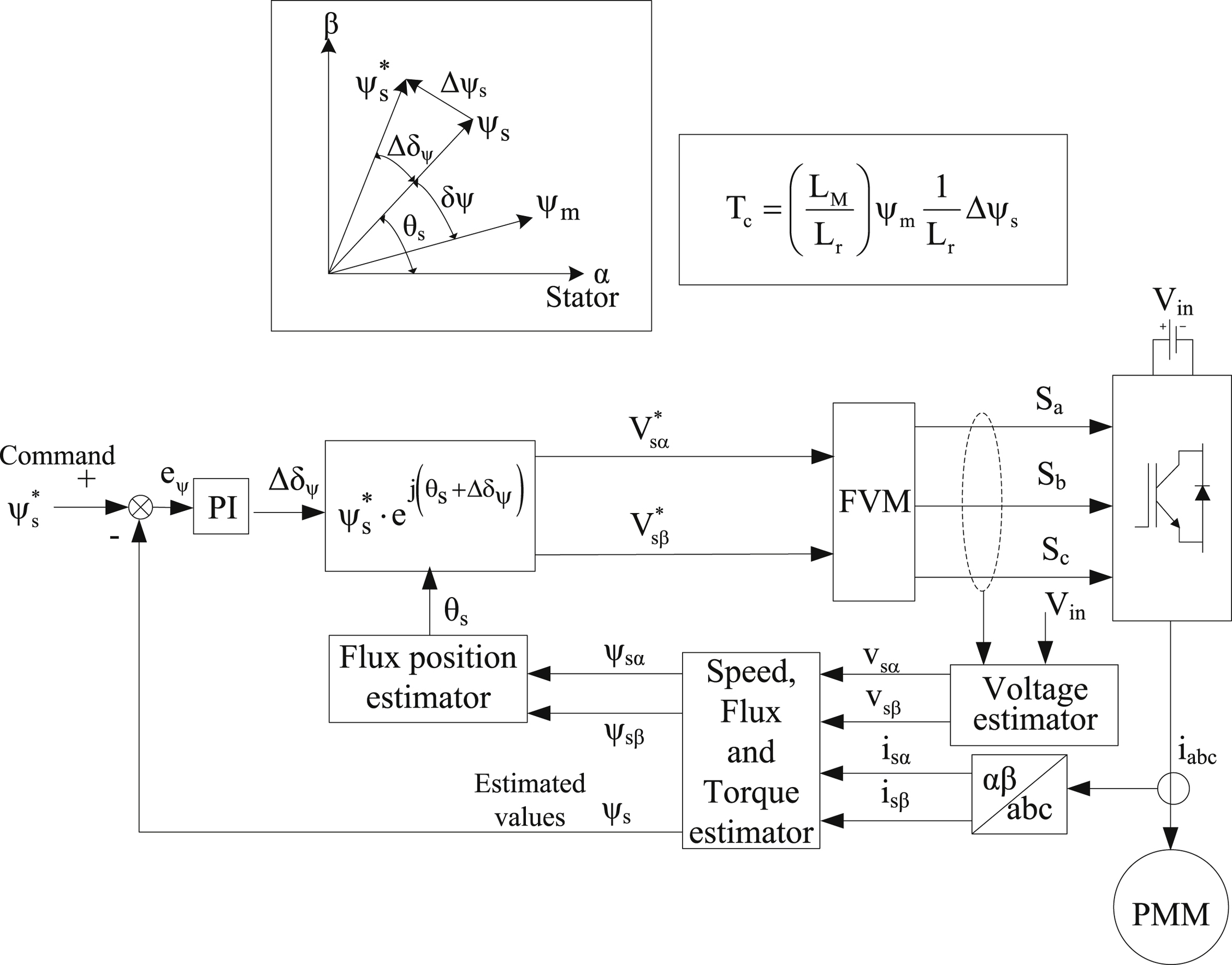
12.5.1.3.5. Direct Torque Control With Flux Vector Modulation (DTC-FVM)
To further simplify the DTC technique, a flux vector modulation (FVM) technique can be utilized, as shown in Fig. 12.66. For the control of the electromagnetic torque, a PI controller is used, whose output produces an increase in the power angle Δδψ (as shown in the vector diagram of Fig. 12.66). Considering that the amplitude of the rotor flux vector remains practically constant, the electromagnetic torque can be controlled by changing the power angle δψ, which corresponds to an increase to the stator flux vector Δψs. The command for the angle of the stator flux vector is calculated as the sum of the estimated position of the field θs and the change in the power angle Δδψ. Its value is compared to the estimated flux and the error signal Δψs is used to directly dictate the switching state of the voltage fed inverter (FVM block). The PI controller of Fig. 12.64 can be omitted, due to the internal stator flux control loop that is used to calculate the change in the flux vector Δψs.
12.5.1.3.6. Nonlinear Torque Control Techniques
Nonlinear controllers adapt the bang–bang control type that is suitable to the switching nature of the operation of the semiconductor switches of the power inverter. In comparison to the FOC, nonlinear DTC controllers exhibit the following characteristics:
• Simple structure
• Absence of current control loops
• Indirect current control
• No need for independent voltage PWM
• No need for speed sensor
• Necessity for accurate estimation of stator flux and torque
In the following section, the most widely used nonlinear control techniques will be analyzed, namely the switching table DTC, the direct self control (DSC) and the online-optimized model-predictive DTC.
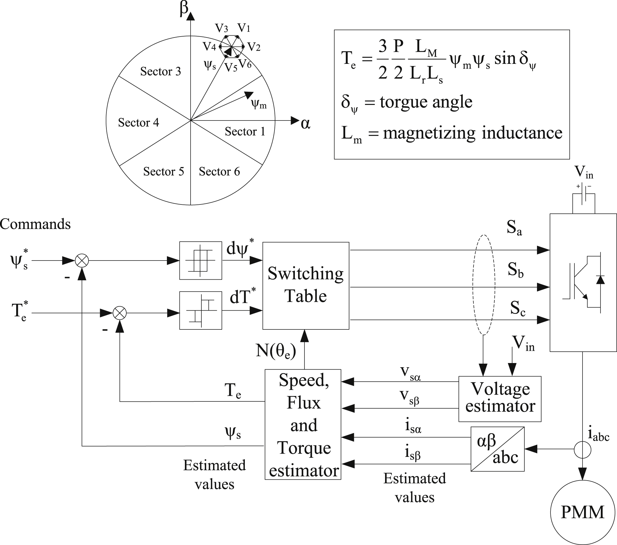
12.5.1.3.7. Switching Table Direct Torque Control (ST-DTC)
The block diagram of the ST-DTC technique is shown in Fig. 12.65. The commands of the stator flux  and the motor torque
  are the signals that are compared to the estimated values ψs and Te, respectively. The error signals that are produced by the hysteresis controllers, dψ and dT, as well as the position sector signal N(θs) of the stator flux vector that is obtained through the calculation of its angular position
  are used to select the suitable voltage vector from the switching table. The latter controls the switching state of the power converter using the signals Sa, Sb, and Sc. The ST-DTC technique has the following operating features:
• Sinusoidal flux and stator current waveforms. The harmonic content is dictated by the tolerance of the respective hysteresis band.
• Excellent dynamic behavior (depending on the voltage level).
• The flux and torque hysteresis bands dictate the switching frequency of the inverter, which varies with the synchronous speed and the load variations.
Over the last decades several modifications of the ST-DTC technique have been proposed to improve the motor transient behavior at start-up, the overload operation, the low speed operation, and the acoustic noise.
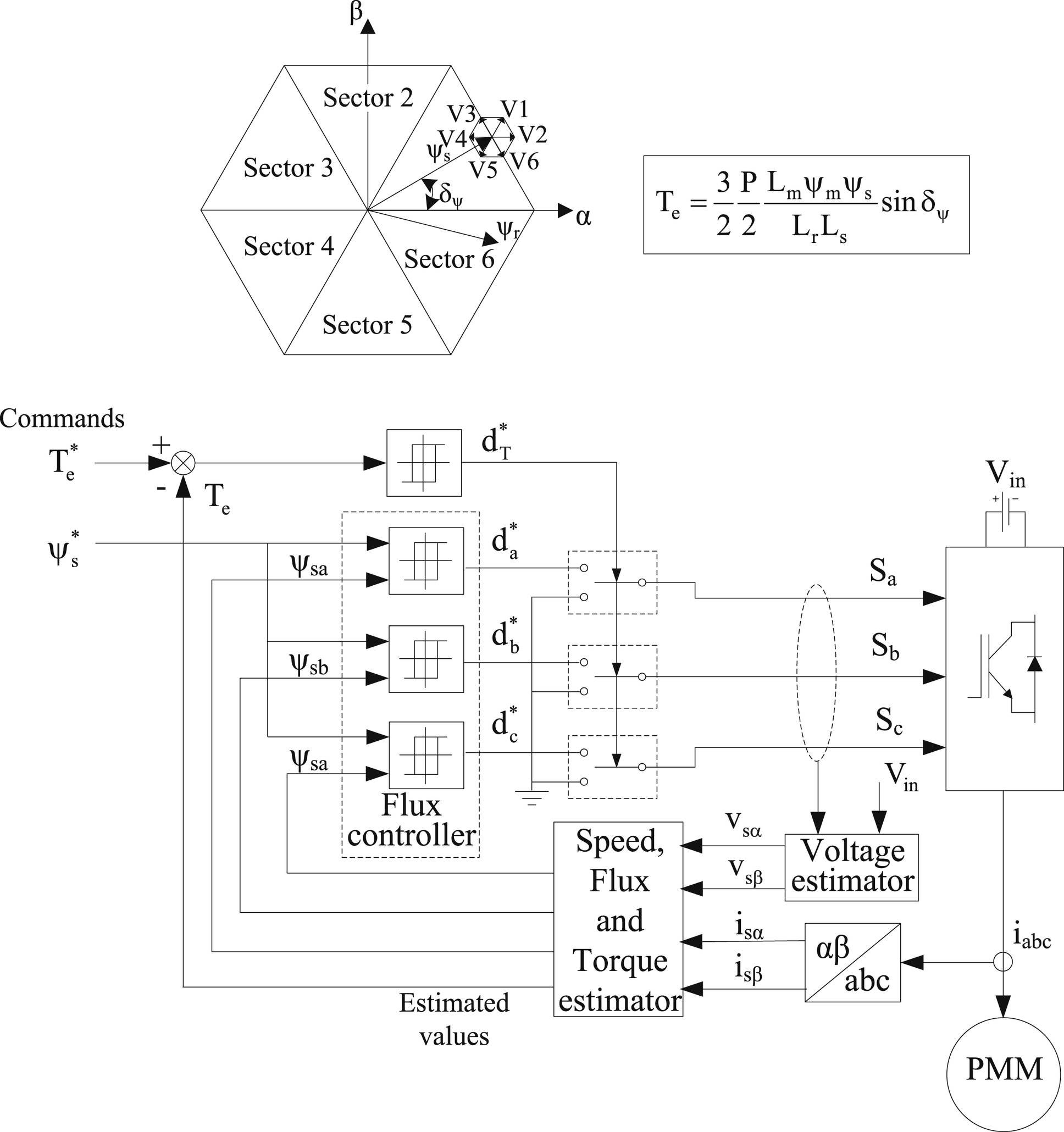
12.5.1.3.8. Direct Self Control (DSC)
The block diagram of the DSC technique is shown in Fig. 12.67. Based on the stator flux command signal ψs∗ and the components ψsa, ψsb, and ψsc, the flux controllers produce the output signals da, db, and dc that correspond to active voltage states (V1–V6). The torque hysteresis controller produces the signal dT that determines the zero voltage states. The flux controller dictates the duration of the active voltage states that implement the defined stator flux orbit. The torque controller dictates the duration of the zero voltage states that maintain the produced torque within the hysteresis band. The DSC technique, as shown in Fig. 12.67, has the following operating features:
• Non-sinusoidal flux and stator current waveforms.
• The locus of the stator flux vector path is an octagon.
• The inverter capability is fully exploited and, consequently, no voltage surplus is required.
• The switching frequency is smaller than the respective of the ST-DTC technique.
• Excellent transient behavior regarding the torque for both constant flux and field weakening operation.
12.5.1.3.9. Online-Optimized Model Predictive Direct Torque Control
The basic principle of predictive control is the utilization of a particular model of the system to be controlled to predict the future behavior of the control variables. This information is used by the controller to calculate the optimum action that will minimize a prescribed cost function. A simplified block diagram of the model-predictive DTC technique is shown in Fig. 12.68. This type of control is called finite control set model predictive control (FCS-MPC), as there are seven available switching states for a two-level voltage source inverter. Contrary to a conventional continuous MPC control operates without a PWM block because the switching state is calculated and optimized online through the minimization of the cost function. In most cases, the cost function is defined as the weighted sum of the torque and flux errors. However, other objectives could be considered, i.e., the reduction of harmonic content, the dc voltage stabilization, etc., that improve the performance of the drive system.
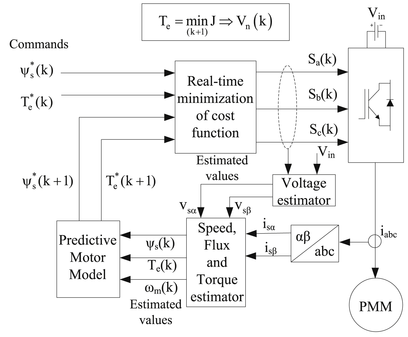
Figure 12.68 Block diagram of the online-optimized model-predictive direct torque and flux control scheme.
The most important advantages of the MPC technique are:
• Ease of implementation.
• Consideration of nonlinearity of the motor model.
• Ease of implementation.
• Adaptability to the demands of the system.
However the implementation of the MPC demands:
• Increased computation power compared to other DTC methods.
• The accuracy of the model strongly affects the performance of the drive system and the quality of the control.
12.5.2. Switched Reluctance Motor (SRM) Drive Systems
RM is defined as the electric motor in which torque is produced form the natural tendency of the moving part (rotor) to rotate towards the position that maximizes the magnetic induction of the excited winding. This definition includes both switched and synchronous RMs. Synchronous RMs comprise a cylindrical rotor with lamination sheets of appropriate configuration, so that it exhibits different magnetic reluctance to each direction, and are generally fed by symmetrical sinusoidal voltages. Switched reluctance motors (SRMs) comprise both a stator and a rotor with salient poles and the name switched derives from the need for switched current feeding to consecutive windings, to achieve continuous rotation. Both of the aforementioned types of electric motors are synchronous and the aforementioned distinction only aims to define the saliency type, i.e., artificial or inherent. For the needs of the analysis undertaken, only SRMs will be investigated and from now on will be referred to as SRM.
12.5.2.1. Description of SRM Structure
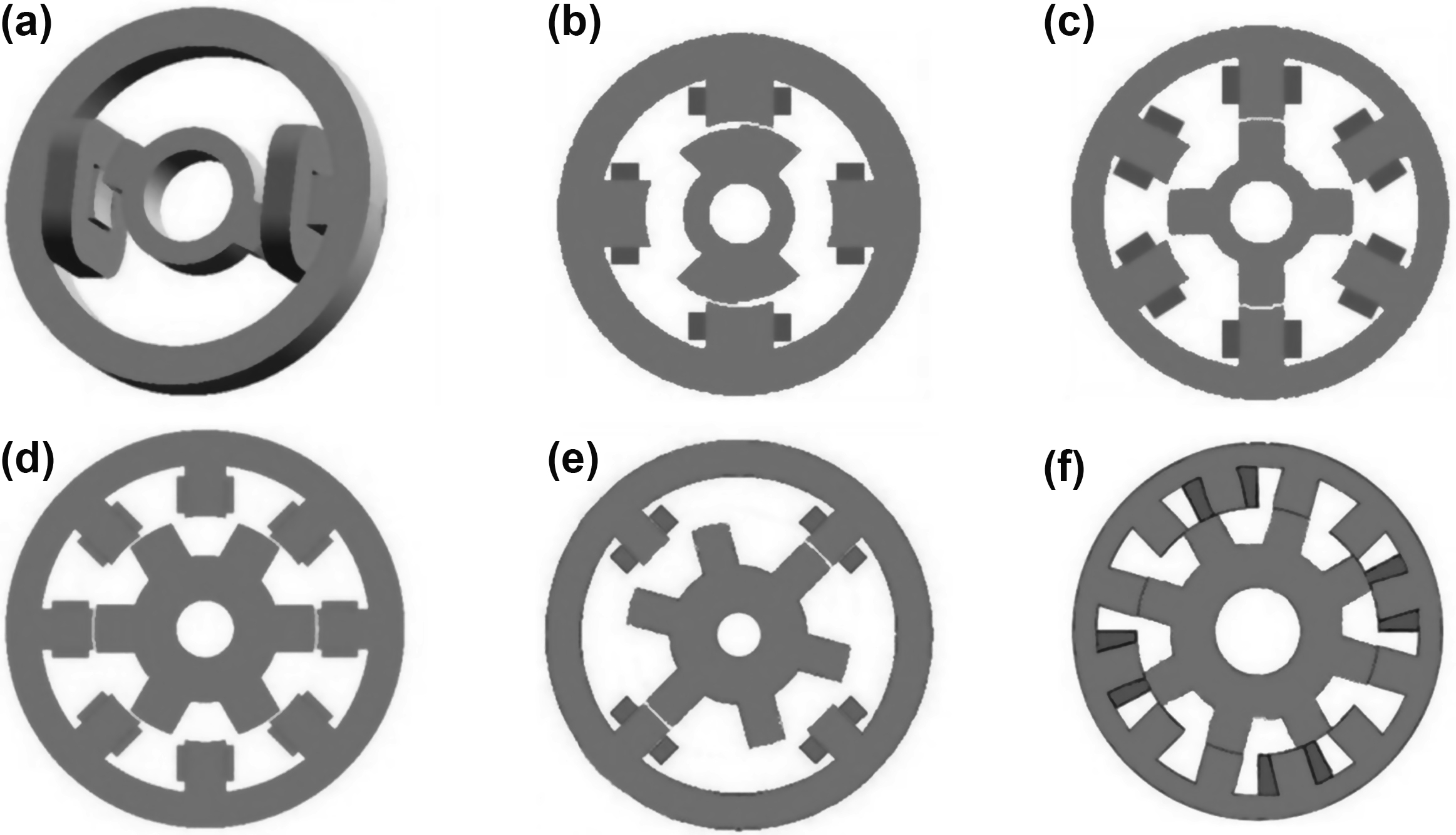
The structure of a variable RM is quite simple. In particular, it consists of a stator with salient poles made of magnetic lamination sheets and a rotor with salient poles, which is, in most cases, also made from conventional magnetic lamination sheets. However, in high performance applications, the lamination sheets are thinner than those normally used in conventional AC motors, and are made from advanced materials like silicon steel sheets, to reduce eddy current losses. The reason is that in an SRM drive system the switching frequency is higher than that of a conventional ac motor drive system of the same dimensions and with the same reference speed. The rotor does not comprise either windings or PMs. The number of stator and rotor poles is inherently different (Ns ≠ Nr), for example, some possible combinations are Ns = 6 and Nr = 4, Ns = 8 and Nr = 6, Ns = 12 and Nr = 10, etc. Such a choice, guarantees that the rotor will never be in a position of zero electromagnetic torque, considering all potential stator winding alternative excitations. The higher the number of stator and rotor poles, the smaller the incurring torque pulsations. By choosing a combination where the number of stator poles is higher than the respective rotor poles by two (one additional pole pair in the stator), a high mean torque value and a low switching frequency in the converter that drives the motor are achieved. It is also possible to select the number of poles so that instead of imposing Ns − Nr = 2, that difference could be negative, so that Ns − Nr = −2, i.e., Ns = 6 and Ns = 8. For the same number of stator poles (Ns), the most important advantage that the higher number of rotor poles (Nr) offers is the smaller step angle and possibly, reduced torque ripple. Such a configuration has the disadvantage of smaller stator pole pitch, resulting in a smaller value of the inductances ratio. The inductances ratio is the ratio of the inductance in aligned position of the stator winding that corresponds to the respective pole to inductance in the not aligned position, and it will be thoroughly analyzed in a following paragraph. In any case, an odd number of stator poles should be avoided, as it alters the balance of the force that act in the motor. It should be noted, that there are viable configurations exhibiting dual teeth on every stator pole, i.e., a motor with six stator poles with two teeth in every pole and a rotor with 10 poles. This can lead to an increase in mean torque per ampere, but consequently will increase magnetization losses. Therefore, such configurations are used in low-speed applications.
The windings of the stator of an SRM are concentrated windings (which are cheaper than the respective distributed). Stator windings of inverse poles (teeth) are connected in series to form a stator phase. Consequently, this way it can be derived that a motor with six stator poles and four rotor poles is actually a three-phase motor (generalized three-phase motor). A motor with Ns = 12, Nr = 8 is also a three-phase motor, but with four stator poles connected in series in every phase. A three-phase motor has the ability to develop electromagnetic torque during starting either towards the positive or the negative rotational direction. If Ns = 2 and Nr = 2, then it is a single-phase motor, but this motor can only be rotated from any given rotor position provided that specific starting options are utilized (i.e., stepped air-gap). If Ns = 4 and Nr = 2, then it's the generalized two-phase motor, which can also be started from any given rotor position only provided that specific starting options are utilized (i.e., stepped air-gap). If Ns = 8 and Nr = 6, then the motor is a four-phase motor, it can be started from any given rotor position and produces smoother electromagnetic torque than the respective three-phase one. Some of the aforementioned configurations are shown in Fig. 12.69.
12.5.2.2. Principles of SRM Operation
The foundation stone of the operation of the SRM is the variable inductance of the windings with the position of the rotor. The rotor moves spontaneously towards positions of increased inductance of the respective winding that is fed, decreasing this way its total mechanical energy (potential that becomes kinetic). The movement of the rotor is actually a repetitive movement between two extreme positions. The first one is the unaligned position, where the magnetic induction (or magnetic flux density) of the winding that is fed is minimum and is a point of unstable equilibrium. The second is called aligned position, and it's the position of maximum magnetic induction for the winding that is fed and is a point of stable equilibrium. The continuous movement is guaranteed through the synchronized excitement of consecutive windings.
To clarify the abovementioned, the simplest case, i.e., the single-phase 2/2 SRM will be analyzed. The motor under analysis is shown in Fig. 12.70. In this figure, the two extreme positions of the rotor are depicted; the aligned position (a) and the unaligned position (b). Additionally, the main characteristics that describe the operation of the SRM are shown. It should be noted, that for the aforementioned characteristics the ideal case of linear operation has been considered. Thus, the nonlinear phenomena of magnetic saturation and magnetic flux leakage around the pole edges have been ignored, and it has been considered that the magnetic flux travels through the air gap in radial paths. We can see that in the aligned position the magnetic flux density of the stator winding takes its maximum value, while in the unaligned position it reaches its minimum value. In practice, when there is no overlap between the poles of the stator and the rotor, the magnetic induction reaches a very small minimum value which is not zero. As soon as the overlapping starts and while moving towards the alignment position, the induction values increase, and in fact in a linear manner. If we consider the fact that during the aforementioned rotor movement the stator windings are constantly excited, then the motor develops the electromagnetic torque that is shown in the second waveform. This can be considered as the possible electromagnetic torque that the motor is capable of producing. We can see that the produced torque takes both positive and negative values, while exhibiting a zero mean value. Apparently, such a torque waveform is far from desired. Consequently, we come to the realization that the stator windings should not be constantly excited, but they should be excited with switched currents depending on the position of the rotor, as shown in the third waveform. The waveform depicts simultaneously the ideal positive current and the consequent ideal positive electromagnetic torque of the motor. However such a tetragonal pulse is not practically feasible. This is mainly due to the fact that the value of the magnetic induction at the start of the pulse is not exactly zero, to achieve rapid current increase, and the fact that the available negative voltage should be infinite to achieve a rapid current interruption. Such an ideal current waveform, in conjunction with the ideal induction waveform, leads to a triangular waveform of the magnetic flux. The ideal torque waveform resembles in shape with the respective current waveform. The torque production cycle, associated with a certain current pulse is called a stroke. Apparently, to produce constant mean torque more than one phases are required, and the mean torque will be produced from the superposition of the respective strokes. Under normal operating conditions, there is a stroke per rotor pole arc for every phase and for each phase current flows only for a fraction of the rotor pole pitch.
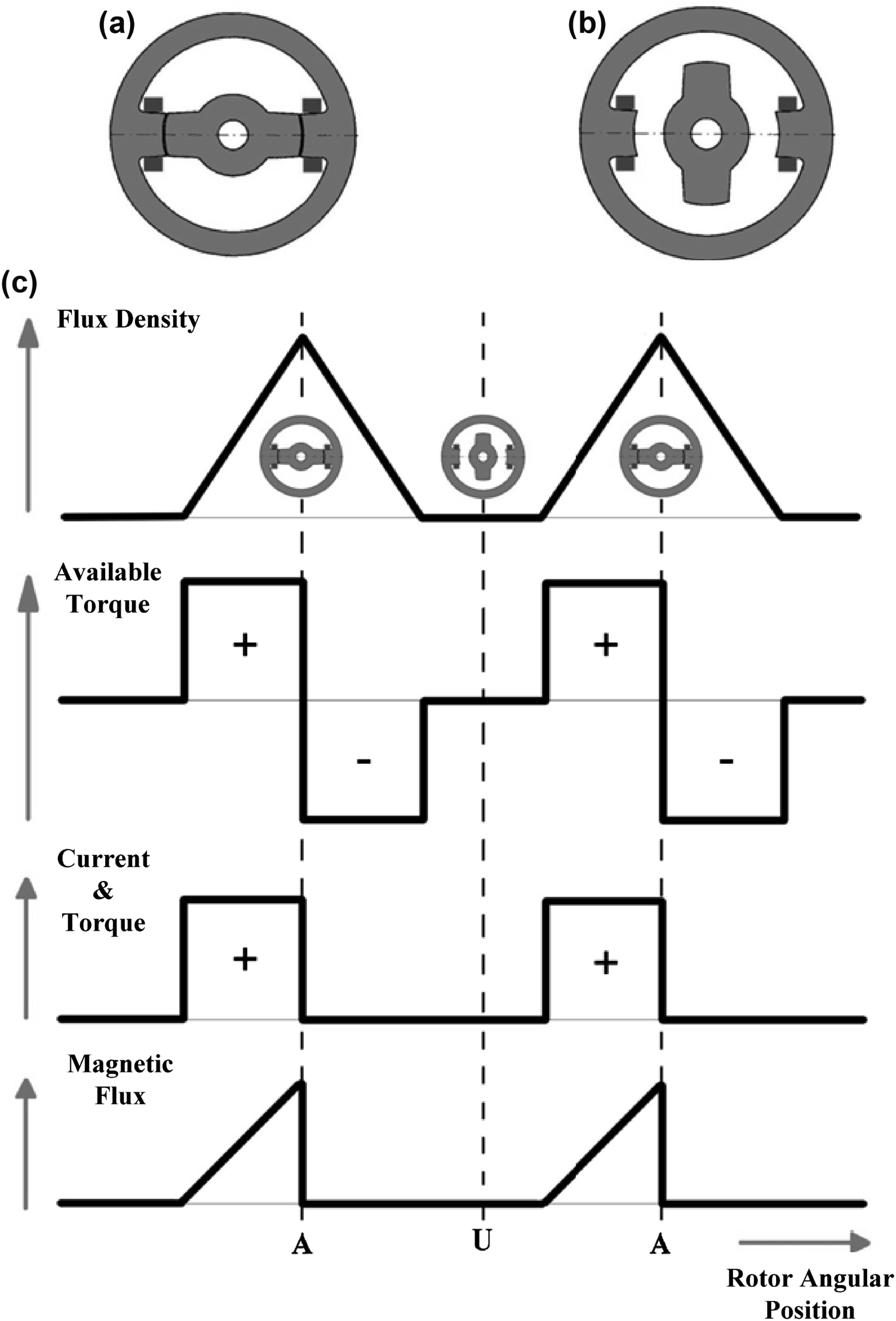
Figure 12.70 Description of the 2/2 switched reluctance motor (SRM).
(a) Aligned rotor position; (b) unaligned rotor position; (c) waveforms related to the ideal operation of a single-phase 2/2 SRM.
Based on the aforementioned analysis, considering a linear magnetic circuit and neglecting the mutual inductances between the windings (which have zero values) the mathematical description of the phase voltages can be derived:
![]() (12.186)
(12.186)
where v and i are the instantaneous values of the voltage and the current of the winding, R is the winding resistance, ψ is the instantaneous value of the magnetic flux, ωm is the mechanical rotational speed, θ is the angular position of the rotor, and L is the inductance of the stator winding. The last term of the equation is called back-EMF of the motor and is given by:
![]() (12.187)
(12.187)
From the above analysis, the equivalent per-phase circuit of the SRM is derived, which is described by Eqs. (12.186) and (12.187). It consists of a resistance connected in series with a variable inductance and a variable back-EMF, as shown in Fig. 12.71.
Therefore, utilizing the visualization of Fig. 12.71, we can distinguish the three voltage terms of Eq. (12.186) in the voltage drop along the winding resistance R, the back-EMF on the variable inductance L, and the velocity back-EMF e, respectively. At this point it should be noted, that the electric equivalent of an SRM is particularly simple as it consists of independent electric circuits, one for each phase, due to the negligible nature of the respective stator mutual inductances. The independence of the electric circuits is a very important characteristic of the SRMs because it facilitates the precise current control and increases the motor's reliability and fault tolerance, as a potential fault in a single phase does not involve the other phases that continue their normal operation. This feature is especially important in applications that require increased reliability or applications where maintenance is difficult.
To fully understand the operation of the SRM, the mathematical description of the torque production mechanism is essential, additionally to the electric equivalent circuit. This procedure will lead to the extraction of the full mathematical model of the SRM. Contrary to the electric equivalent circuit, the description of the aforementioned mechanism is particularly difficult, because of the complex nonlinear electromagnetic phenomena related to it. Initially, a simplified linear approach shall be made, which will produce results adequately close to the real motor behavior.
From Eq. (12.186), the per-phase instantaneous electric power of an SRM is derived:
![]() (12.188)
(12.188)
Considering a linear magnetic circuit and neglecting hysteresis and eddy currents, the instantaneous stored magnetic power of the magnetic circuit is given by equation:
![]() (12.189)
(12.189)
According to the law of conservation of energy, electric power finally changing to mechanical is derived from the circuit input power, if the ohmic thermal losses on the resistance R and the instantaneous power stored in the magnetic circuit are subtracted:
![]() (12.190)
(12.190)
where Te is the instantaneous electromagnetic torque of each phase of the SRM.
Consequently, by solving Eq. (12.190) we obtain:
![]() (12.191)
(12.191)
where dL/dθ is the slope of the magnetic flux density waveform, shown in Fig. 12.70(c). It should be mentioned that for the analysis undertaken, linear magnetic circuit and ideal operational characteristics of the motor are considered, as shown in Fig. 12.70(c). From Eq. (12.191) fundamental conclusions regarding the nature and the operation of the SRM can be deducted. First, it can be concluded that the sign of the produced electromagnetic torque does not depend on the sign of the phase current, because it is proportional to the square of the current value, as shown from Eq. (12.191). That means that unidirectional currents are necessary for the operation of such a motor, something that significantly simplifies the driving converter configuration. Second, it can be concluded that the sign of the produced electromagnetic torque only depends on the sign of the term dL/dθ, namely the slope of the magnetic flux density waveform. If we take a closer look at the ideal waveform of flux density, shown in Fig. 12.70(c), it becomes apparent that the slope is initially positive and then becomes negative. Consequently, the electromagnetic torque, shown in Fig. 12.70(c), changes sign exactly at the point that the magnetic flux density slope changes. This practically means that if a positive electromagnetic torque is desired, the winding should be excited only during the time when the magnetic flux density is increasing and the excitation should stop as soon as its values starts decreasing, as shown in Fig. 12.70(c). For the aforementioned analysis a nonrealistic consideration of linearity of the magnetic circuit is employed.
12.5.2.3. Power Electronics Converter for SRM Drive Systems
Various different power electronic converters have been proposed for SRM drive systems that meet the aforementioned requirements. The simplest and most often used converter for that purpose is the single-phase asymmetrical voltage source inverter, which is shown in Fig. 12.72. The converter is fed by a dc voltage source Vdc and comprises two semiconductor switches (S1 and S2) and two diodes (D1 and D2).
The load of the converter is the stator winding of a phase of the SRM. Therefore, a number of converters equal to the number of the phases of the SRM are required. It is possible to reduce the number of the semiconductor switches through the merging of specific legs of the converters. However, this could result in decreased reliability due to the fact that it cancels the modularity of the converter, as if one phase has a fault the others are unable to normally operate. Therefore, a single-phase asymmetrical inverter per-phase is used in most applications, as shown in Fig. 12.72. Additionally, in practice, as will be revealed by the following analysis, only a single semiconductor switch per-phase is actually necessary. Consequently, the second switch can be replaced by a diode. The drawback of this option is the inability to achieve equal use of all the switches and even distribution of their respective losses. This is a major disadvantage that is usually evaluated as of higher significance than the extra cost of a semiconductor switch compared to that of a diode. The overall converter for a three-phase SRM drive comprises the same number of switches with a typical three-phase inverter, while rendering its potential reduction feasible. However, the establishment of the three-phase inverters as standard driving systems and their wide production renders them more economical than a respective SRM converter.
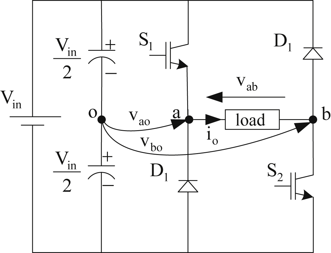
In the following paragraph, the operation of the single-phase asymmetrical voltage source inverter will be analyzed in detail and its mathematical model will be extracted. In Fig. 12.73, all possible switching states of the converter are shown.
From the above analysis, it becomes apparent that such a converter is able to drive an SRM, as it allows the production of both positive and negative voltage and unidirectional currents. The mathematical model of the converter, which fully describes its operational states, is shown below. The various switching states shown in Fig. 12.73, can be analytically described using the following equation:
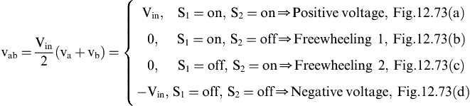 (12.192)
where the variables va and vb are defined by the switching state of the semiconductor switches S1 and S2 as follows:
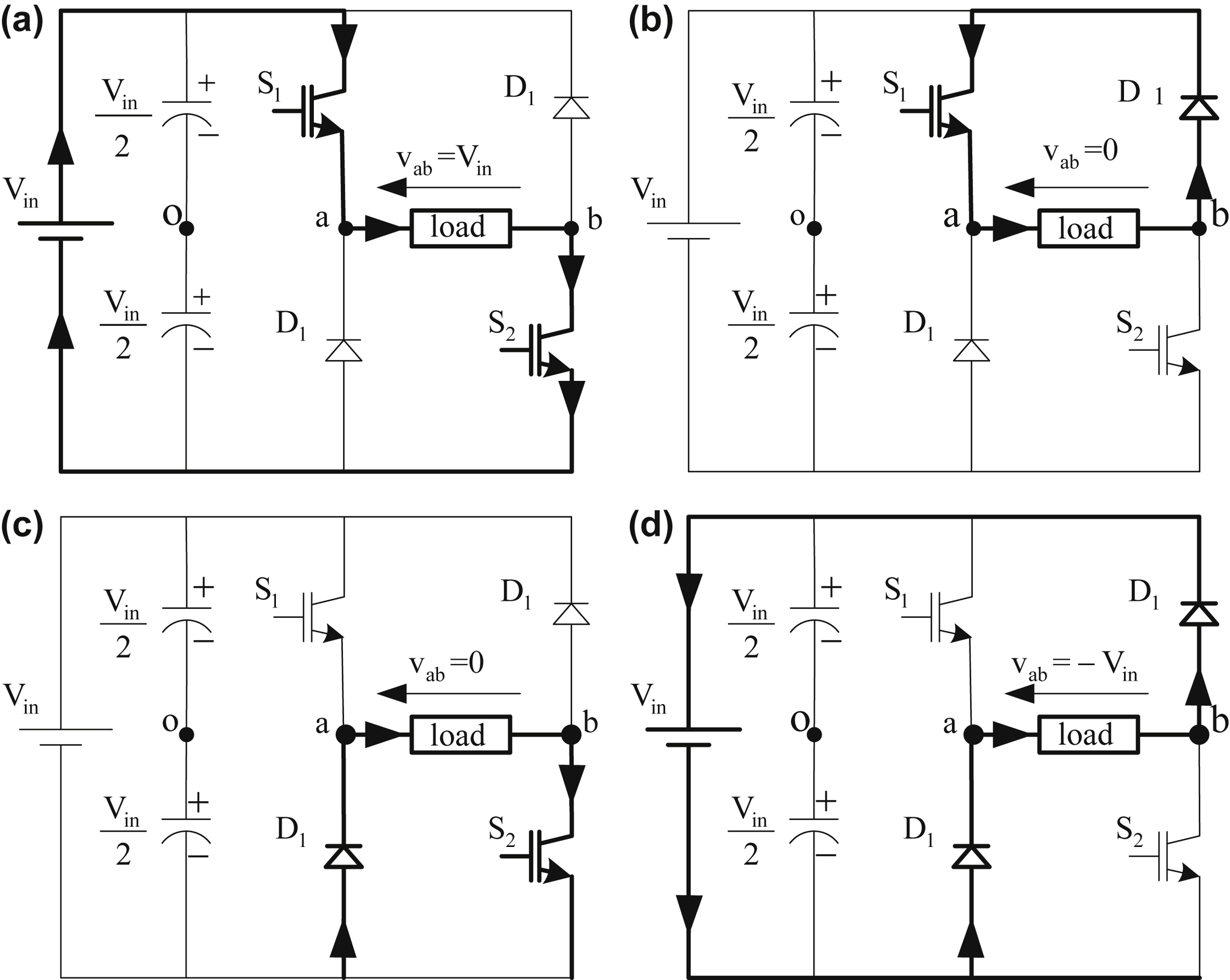
Figure 12.73 Possible switching states and the respective output voltages of the converter.
(a) Both switches (S1 and S2) are conducting and positive voltage is applied to the load; (b) one switch (S1) and a diode (D2) are conducting, short-circuiting the load (freewheeling); (c) one switch (S2) and a diode (D1) are conducting, short-circuiting the load (freewheeling); (d) none of the switches is conducting and negative voltage is applied to the load through the diodes (D1 and D2).
 (12.193)
 (12.194)
Eq. (12.192) combined with Eqs. (12.193) and (12.194) comprise the simplified mathematical model of the single-phase asymmetrical voltage source inverter that is used to drive an SRM.
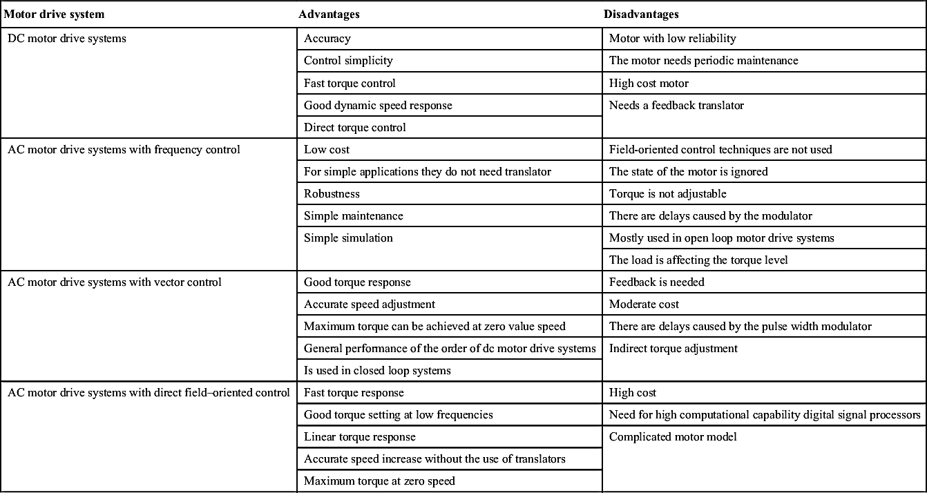
Table 12.8
Comparison between different motor drive systems
| Motor drive system | Advantages | Disadvantages |
| DC motor drive systems | Accuracy | Motor with low reliability |
| Control simplicity | The motor needs periodic maintenance | |
| Fast torque control | High cost motor | |
| Good dynamic speed response | Needs a feedback translator | |
| Direct torque control | ||
| AC motor drive systems with frequency control | Low cost | Field-oriented control techniques are not used |
| For simple applications they do not need translator | The state of the motor is ignored | |
| Robustness | Torque is not adjustable | |
| Simple maintenance | There are delays caused by the modulator | |
| Simple simulation | Mostly used in open loop motor drive systems | |
| The load is affecting the torque level | ||
| AC motor drive systems with vector control | Good torque response | Feedback is needed |
| Accurate speed adjustment | Moderate cost | |
| Maximum torque can be achieved at zero value speed | There are delays caused by the pulse width modulator | |
| General performance of the order of dc motor drive systems | Indirect torque adjustment | |
| Is used in closed loop systems | ||
| AC motor drive systems with direct field–oriented control | Fast torque response | High cost |
| Good torque setting at low frequencies | Need for high computational capability digital signal processors | |
| Linear torque response | Complicated motor model | |
| Accurate speed increase without the use of translators | ||
| Maximum torque at zero speed |
..................Content has been hidden....................
You can't read the all page of ebook, please click here login for view all page.