8

Exploring Optional Parameters for H2O AutoML

As we explored in Chapter 2, Working with H2O Flow (H2O’s Web UI), when training models using H2O AutoML, we had plenty of parameters to select. All these parameters gave us the capability to control how H2O AutoML should train our models. This control helps us get the best possible use of AutoML based on our requirements. Most of the parameters we explored were pretty straightforward to understand. However, there were some parameters whose purpose and effects were slightly complex to be understood at the very start of this book.

In this chapter, we shall explore these parameters by learning about the Machine Learning (ML) concepts behind them, and then understand how we can use them in an AutoML setting.

By the end of this chapter, you will not only be educated in some of the advanced ML concepts, but you will also be able to implement them using the parametric provisions made in H2O AutoML.

In this chapter, we will cover the following topics:

• Experimenting with parameters that support imbalanced classes
• Experimenting with parameters that support early stopping
• Experimenting with parameters that support cross-validation

We will start by understanding what imbalanced classes are.

Technical requirements

You will require the following to complete this chapter:

• The latest version of your preferred web browser.
• The H2O software installed on your system. Refer to Chapter 1, Understanding H2O AutoML Basics, for instructions on how to install H2O on your system.

Tip

All the H2O AutoML function parameters shown in this chapter are shown using H2O Flow to keep things simple. The equivalent parameters are also available in the Python and R programming languages for software engineers to code into their services. You can find these details at https://docs.h2o.ai/h2o/latest-stable/h2o-docs/parameters.html.

Experimenting with parameters that support imbalanced classes

One common problem you will often face in the field of ML is classifying rare events. Consider the case of large earthquakes. Large earthquakes of magnitude 7 and higher occur about once every year. If you had a dataset containing the Earth’s tectonic activity of each day since the last decade with the response column containing whether or not an earthquake occurred, then you would have approximately 3,650 rows of data; that is, one row for each day in the decade, with around 8-12 rows showing large earthquakes. That is less than a 0.3% chance that this event will occur. 99.7% of the time, there will be no large earthquakes. This dataset, where the number of large earthquake events is so small, is called an imbalanced dataset.

The problem with the imbalanced dataset is that even if you write a simple if-else function that marks all tectonic events as not earthquakes and call this a model, it will still show the accuracy as 99.7% accuracy since the majority of the events are not earthquake-causing. However, in actuality, this so-called model is very bad as it is not correctly informing you whether it is an earthquake or not.

Such imbalance in the target class creates a lot of issues when training ML models. The ML models are more likely to assume that these events are so rare that they will never occur and will not learn the distinction between those events.

However, there are ways to tackle this issue. One way is to undersample the majority class and the other way is to oversample the minority class. We shall learn more about these techniques in the upcoming sections.

Understanding undersampling the majority class

In the scenario of predicting the occurrence of earthquakes, the dataset contains a large number of events that have been identified as not-earthquake. This event is known as the majority class. The few events that mark the activity as an earthquake are known as the minority class.

Let’s see how undersampling the majority class can solve the problems caused by an imbalance in the classes. Consider the following diagram:

Figure 8.1 – Undersampling an imbalanced dataset

Let’s assume you have 3,640 data samples of tectonic activity that indicate no earthquakes happened and only 10 samples that indicate earthquakes happened. In this case, to tackle this imbalance issue, you must create a bootstrapped dataset containing all 10 samples of the minority class, and 10 samples of the majority class chosen at random from the 3,640 data samples. Then, you can feed this new dataset to H2O AutoML for training. In this case, we have undersampled the majority class and equalized the earthquake and not-earthquake data samples before training the model.

The drawback of this approach is that we end up tossing away huge amounts of data, and the model won’t be able to learn a lot from the reduced data.

Understanding oversampling the minority class

The second approach to tackling the imbalanced dataset issue is to oversample the minority class. One obvious way is to duplicate the minority class data samples and append them to the dataset so that the number of data samples between the majority and minority classes is equal. Refer to the following diagram for a better understanding:

Figure 8.2 – Oversampling an imbalanced dataset

In the preceding diagram, you can see that we replicated the minority class data samples and appended them to the dataset so that we ended up with 3,640 rows for each of the classes.

This approach can work; however, oversampling will lead to an explosion in the size of the dataset. You need to make sure that it does not exceed your computation and memory limits and end up failing.

Now that we’ve covered the basics of class balancing using undersampling and oversampling, let’s see how H2O AutoML handles it using its class balancing parameters.

Working with class balancing parameters in H2O AutoML

H2O AutoML has a parameter called balance_classes that accepts a boolean value. If set to True, H2O performs oversampling on the minority class and undersampling on the majority class. The balancing is performed in such a way that eventually, each class contains the same number of data samples.

Both undersampling and oversampling of the respective classes is done randomly. Additionally, oversampling of the minority class is done with replacement. This means that data samples from the minority class can be chosen and added to the new training dataset multiple times and can be repeated.

H2O AutoML has the following parameters that support class balancing functionality:

• balance_classes: This parameter accepts a boolean value. It is False by default, but if you want to perform class balancing on your dataset before feeding it to H2O AutoML for training, then you can set the boolean value to True.

In H2O Flow, you get a checkbox besides the parameter. Refer to the following screenshot:

Figure 8.3 – The balance_classes checkbox in H2O Flow

Checking it makes the class_sampling_factors and max_after_balance_size parameters available in the EXPERT section of the Run AutoML parameters, as shown in the following screenshot:

Figure 8.4 – The class_sampling_factors and max_after_balance_size parameters in the EXPERT section

• class_sampling_factors: This parameter requires balance_classes to be True. This parameter takes a list of float values as input that will represent the sampling rate for that class. A sampling rate of value 1.0 for a given class will not change its sample rate during class balancing. A sampling rate of 0.5 will halve the sample rate of a class during class balancing while a sampling rate of 2.0 will double it.
• max_after_balance_size: This parameter requires balance_classes to be True and specifies the maximum relative size of the training dataset after balancing. This parameter accepts a float value as input, which would limit the size your training dataset can grow to. The default value is 5.0, which indicates that the training dataset will grow a maximum of 5 times its size. This value can also be less than 1.0.

In the Python programming language, you can set these parameters as follows:

aml = h2o.automl.H2OAutoML(balance_classes = True, class_sampling_factors =[0.3, 2.0], max_after_balance_size=0.95, seed = 123)
aml.train(x = features, y = label, training_frame = train_dataframe)

Similarly, in the R programming language, you can set these parameters as follows:

aml <- h2o.automl(x = features, y = label, training_frame = train_dataframe, seed = 123, balance_classes = TRUE, class_sampling_factors = c(0.3, 2.0), max_after_balance_size=0.95)

To perform class balancing when training models using AutoML, you can set the balance_classes parameter to true in the H2O AutoML estimator object. In that same object, you can specify your class_sampling_factors and max_after_balance_size parameters. Then, you can use this initialized AutoML estimator object to trigger AutoML on your training dataset.

Now that you understand how we can tackle the class imbalance issue using the balance_classes, class_sampling_factors, and max_after_balance_size parameters, let’s understand the next optional parameters in AutoML – that is, stopping criteria.

Experimenting with parameters that support early stopping

Overfitting models is one of the common issues often faced when trying to solve an ML problem. Overfitting is said to have occurred when the ML model tries to adapt to your training set too much, so much so that it is only able to make predictions on values that it has seen before in the training set and is unable to make a generalized prediction on unseen data.

Overfitting occurs due to a variety of reasons, one of them being that the model learns so much from the dataset that it even incorporates and learns the noise in the dataset. This learning negatively impacts predictions on new data that may not have that noise. So, how do we tackle this issue and prevent the model from overfitting? Stop the model early before it learns the noise.

In the following sub-sections, we shall understand what early stopping is and how it is done. Then, we will learn how the early stopping parameters offered by H2O AutoML work.

Understanding early stopping

Early stopping is a form of regularization that stops a model’s training once it has achieved a satisfactory understanding of the data and further prevents it from overfitting. Early stopping aims to observe the model’s performance as it improves using an appropriate performance metric and stop the model’s training once deterioration is observed due to overfitting.

When training a model using algorithms that use iterative optimization to minimize the loss function, the training dataset is passed through the algorithm during each iteration. Observations and understandings that pass are then used during the next iteration. This iteration of passing the training dataset through the algorithm is called an epoch.

For early stopping, at the end of every epoch, we can calculate the performance of the model and note down the metric value. Comparing these values during every iteration helps us understand whether the model is improving its performance after every epoch or whether it is learning noise and losing performance. We can monitor this and stop the model training at the epoch where we start seeing a decrease in performance. Refer to the following diagram to gain a better understanding of early stopping:

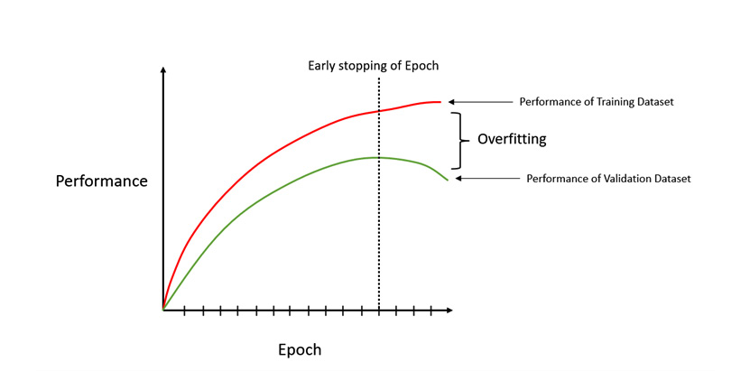
Figure 8.5 – Early stopping to avoid model overfitting

In the preceding diagram, on the Y axis, we have the Performance value of the model. On the X-axis, we have the Epoch value. So, as time goes on and we iterate through the number of epochs, we see that the performance of the model on the training set and the validation set continues to increase. But after a certain point, the performance of the model on the validation dataset starts decreasing, while the performance of the training dataset continues to increase. This is where overfitting starts. The model learns too much from the training dataset and starts incorporating noise into its learning. This might show high performance on the training dataset, but the model fails to generalize the predictions. This leads to bad predictions on unseen data, such as the ones in the validation dataset.

So, the best thing to do is to stop the model at the exact point where the performance of the model is highest for both the training and validation dataset.

Now that we have a basic understanding of how early stopping of model training works, let’s learn how we can perform it using the early stopping parameter offered by the H2O AutoML function.

Working with early stopping parameters in H2O AutoML

H2O AutoML has provisions for you to implement and control the early stopping of your models that it will auto train for you.

You can use the following parameters to implement early stopping:

• stopping_rounds: This parameter indicates the number of training rounds over which if the stopping metric fails to improve, we stop the model training.
• stopping_metric: This parameter is used to select the performance metric to consider when early stopping. It is available if stopping_rounds is set and is greater than 0. We studied performance metrics in Chapter 6, Understanding H2O AutoML Leaderboard and Other Performance Metrics, so kindly refer to that chapter if you wish to revise how the different metrics measure performance. The available options for this parameter are as follows:
  • AUTO: This is the default value and further defaults to the following values, depending on the type of ML problem:
    • logloss: The default stopping metric for classification problems.
    • deviance: The default stopping metric for regression problems. This stands for mean residual deviance.
    • anomaly_score: The default stopping metric for Isolation Forest models, which are a type of ensemble model.
  • anomaly_score: The default stopping metric for Isolation Forest models (ensemble models). It is the measure of normality of an observation equivalent to the number of splits in a decision tree needed to isolate a point in a given tree where that point is at max depth.
  • deviance: This stands for mean residual deviance. This value tells us how well the label value can be predicted by a model based on the number of features in the dataset.
  • logloss: Log loss is a metric that is a way of measuring the performance of a classification model that outputs classification results in the form of probability values.
  • MSE (Mean Squared Error): This is a metric that measures the mean of the squares of errors of the predicted value against the actual value.
  • RMSE (Root Mean Squared Error): This is a metric that calculates the root value of the MSE.
  • MAE (Mean Absolute Error): This is a metric that calculates the average magnitude of errors in each set of observations.
  • RMSLE (Root Mean Squared Logarithmic Error): This is a metric that calculates the RMSE of the log-transformed observed and log-transformed actual values.
  • AUC (Area Under the ROC Curve): AUC-ROC is a metric that helps us compare which classification algorithm performed better, depending on whose ROC curve covers the most area.
  • AUCPR (Area Under the Precision-Recall Curve): AUCPR is similar to the AUC-ROC curve, with the only difference being that the PR curve is a function that uses precision on the Y axis and recall on the X axis.
  • lift_top_group: This parameter configures AutoML in such a way that the model being trained must improve its lift within the top 1% of the training data. Lift is nothing but the measure of performance of a model in making accurate predictions, compared to a model that randomly makes predictions. The top 1% of the dataset are the observations with the highest predicted values.
  • misclassification: This metric is used to measure the fraction of the predictions that were incorrectly predicted without distinguishing between positive and negative predictions.
  • mean_per_class_error: This is a metric that calculates the average of all errors per class in a dataset containing multiple classes.
  • custom: This parameter is used to set any custom metric as the stopping metric during AutoML training. The custom metric should be of the behavior less is better, meaning the lower the value of the custom metric, the better the performance of the model. The lower bound value of the custom metric is assumed to be 0.
  • custom_increasing: This parameter is for custom performance metrics that have the behavior as more is better, meaning the higher the value of these metrics, the better the model performance. At the time of writing, this parameter is only supported in the Python client for GBM and DRF.
• stopping_tolerance: This parameter indicates the tolerance value by which the model’s performance metric must improve before stopping the model training. It is available if stopping_rounds is set and is greater than 0. The default stopping tolerance for AutoML is 0.001 if the dataset contains at least 1 million rows; otherwise, the value is determined by the size of the dataset and the amount of non-NA data in the dataset, which leads to a value greater than 0.001

In H2O Flow, these parameters are available in the ADVANCED section of the Run AutoML parameters, as shown in the following screenshot:

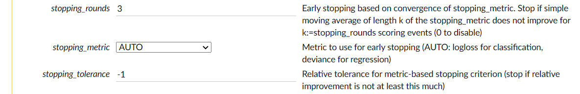
Figure 8.6 – Early stopping parameters in H2O Flow

In the Python programming language, you can set these parameters as follows:

aml = h2o.automl.H2OAutoML(stopping_metric = "mse", stopping_rounds = 5, stopping_tolerance = 0.001)

aml.train(x = features, y = label, training_frame = train_dataframe)

In the R programming language, you can set these parameters as follows:

aml <- h2o.automl(x = features, y = label, training_frame = train_dataframe, seed = 123, stopping_metric = "mse", stopping_rounds = 5, stopping_tolerance = 0.001)

To better understand how AutoML will stop a model's training early, consider the same Python and R example values. We have stopping_metric as mse, stopping_rounds as 5, and stopping_tolerance as 0.001.

When implementing early stopping, H2O will calculate the moving average of the last 6 stopping rounds, where the average of the very first round is used as a reference for the next rounds. If the ratio between the best moving average and the reference moving average is greater than or equal to a stopping_tolerance of 0.001, then H2O will stop the model training. For performance metrics that have the more is better behavior, the ratio between the best moving average and reference moving average should be less than or equal to the stopping tolerance.

Now that we understand how to stop model training early using the stopping_rounds, stopping_metrics, and stopping tolerance parameters, let’s understand the next optional parameter in AutoML – that is, cross-validation.

Experimenting with parameters that support cross-validation

When performing model training on a dataset, we usually perform a train-test split on the dataset. Let’s assume we split it in the ratio of 70% and 30%, where 70% is used to create the training dataset and the remaining 30% is used to create the test dataset. Then, we pass the training dataset to the ML system for training and use the test dataset to calculate the performance of the model. A train-test split is often performed in a random state, meaning 70% of the data that was used to create the training dataset is often chosen at random from the original dataset without replacement, except in the case of time-series data, where the order of the events needs to be maintained or in the case where we need to keep the classes stratified. Similarly, for the test dataset, 30% of the data is chosen at random from the original dataset to create the test dataset.

The following diagram shows how data from the dataset is randomly picked to create the training and testing datasets for their respective purposes:

Figure 8.7 – Train-test split on the dataset

Now, the issue with the train-test split is that when 30% of the data kept outside the testing dataset is not used to train the model, any missing knowledge that could be derived from this data isn’t available to train the model. This leads to a loss in the performance of the model. If you retrain a model using a different random state for the train-test split, then the model will end up having a different performance level as it has been trained on different data records. Thus, the performance of the models depends on the random assignment of the training dataset. So, how can we provide the test data for training as well as keeping some test data for performance measurement? This is where cross-validation comes into play.

Understanding cross-validation

Cross-validation is a model validation technique that resamples data to train and test models. The technique uses different parts of the dataset for training and testing during each iteration. Multiple iterations of model training and testing are performed using different parts of the dataset. The performance results are combined to give an average estimation of the model’s performance.

Let’s try to understand this with an example. Let’s assume your dataset contains around 1,000 records. To perform cross-validation, you must split the dataset into a ratio – let’s assume a 1:9 ratio where we have 100 records for the test dataset and 900 records for the training dataset. Then, you perform model training on the training dataset. Once the model has been trained, you must test the model on the test dataset and note its performance. This is your first iteration of cross-validation.

In the next iteration, you split the dataset in the same ratio of 1/9 records for the testing and training datasets, respectively, but this time, you choose different data records to form your test dataset and use the remaining records as the training dataset. Then, you perform model training on the training dataset and calculate the model’s performance on the testing dataset. You repeat the same experiment using different data records until all the dataset has been used for training as well as testing. You will need to perform around 10 iterations of cross-validation so that, during the entire cross-validation process, the model is trained and tested on the entire dataset each iteration while containing different data records in the testing DataFrame.

Once all the iterations have finished, you must combine the performance results of the experiments and provide the average estimation of the model’s performance. This technique is called cross-validation.

You may have noticed that during cross-validation, we perform model training multiple times on the same dataset. This is expected to increase the overall ML process time. This is especially true when performing cross-validation on a large dataset with a very high ratio between the training and testing partition. For example, if we have a dataset that contains 30,000 rows and we split the dataset into 29,000 rows for training and 1,000 rows for testing, then this will lead to a total of 3,000 iterations of model training and testing. Hence, there is an alternative form of cross-validation that lets you choose how many iterations to perform: called K-fold cross-validation.

In K-fold cross-validation, you decide the value of K, which is used to determine the number of cross-validation iterations to perform. Depending on the value of K, the ML service will randomly partition the dataset into K equal subsamples that will be resampled over the cross-validation iterations. The following diagram will help you understand this:

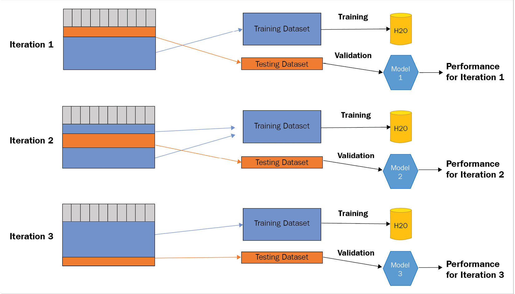
Figure 8.8 – K-fold cross-validation where K=3

As you can see, we have a dataset that contains 30,000 data records and the chosen value of K in the K-fold cross-validation is 3. Accordingly, the dataset will be split into 20,000 records for the test dataset and 10,000 records for training, which will be resampled during the following iterations, leading to a total of three cross-validations.

The benefit of using K-fold cross-validation to perform your model validation is that the model is trained on the entire dataset without missing out on data during training. This is especially beneficial in multi-class classification problems where there are chances that the model might miss out training on some of the prediction classes because it got split out from the training dataset to be used in the testing dataset.

Now that we have a better understanding of the basics of cross-validation and how it works, let’s see how we can perform it using special parameters in the H2O AutoML training function.

Working with cross-validation parameters in H2O AutoML

H2O AutoML has provisions for you to implement K-fold cross-validation on your data for all ML algorithms that support it, along with some additional information that may help support the implementation.

You can use the following parameters to implement cross-validation:

• nfolds: This parameter sets the number of folds to use for K-fold cross-validation.

In H2O Flow, this parameter will be available in the ADVANCED section of the Run AutoML parameters, as shown in the following screenshot:

Figure 8.9 – The nfolds parameter in H2O Flow

• fold_assignment: This parameter is used to specify the fold assignment scheme to use to perform K-fold cross-validation. The various types of fold assignments you can set are as follows:
  • AUTO: This assignment value lets the model training algorithm choose the fold assignment to use. AUTO currently uses Random as the fold assignment.
  • Random: This assignment value is used to randomly split the dataset based on the nfolds value. This value is set by default if nfolds > 0 and fold_column is not specified.
  • Modulo: This assignment value is used to perform a modulo operation when splitting the folds based on the nfolds value.
  • Stratified: This assignment value is used to arrange the folds based on the response variable for classification problems.

In the Python programming language, you can set these parameters as follows:

aml = h2o.automl.H2OAutoML(nfolds = 10, fold_assignment = "AUTO", seed = 123)

aml.train(x = features, y = label, training_frame = train_dataframe)

In the R programming language, you can set these parameters as follows:

aml <- h2o.automl(x = features, y = label, training_frame = train_dataframe, seed = 123, nfolds = 10, fold_assignment = "AUTO")

• fold_column: This parameter is used to specify the fold assignment based on the contents of a column rather than any procedural assignment technique. You can custom set the fold values per row in the dataset by creating a separate column containing the fold IDs and then setting fold_column to the custom column’s name.

In H2O Flow, this parameter will be available in the ADVANCED section of the Run AutoML parameters, as shown in the following screenshot:

Figure 8.10 – The fold_column parameter in H2O Flow

In the Python programming language, you can set these parameters as follows:

aml.train(x = features, y = label, training_frame = train_dataframe, fold_column = "fold_column_name")

In the R programming language, you can set these parameters as follows:

aml <- h2o.automl(x = features, y = label, training_frame = train_dataframe, seed = 123, fold_column="fold_numbers")

• keep_cross_validation_predictions: When performing K-fold cross-validation, H2O will train K+1 number of models, where K number of models are trained as a part of cross-validation and 1 additional model is trained on the entire dataset. Each of the cross-validation models makes predictions on the test DataFrame for that iteration and the predicted values are stored in a prediction frame. You can save these prediction frames by setting this parameter to True. By default, this parameter is set to False.
• keep_cross_validation_models: Similar to keep_cross_validation_predictions, you can also choose to keep the models trained during cross-validation for further inspection and experimentation by enabling this parameter to True. By default, this parameter is set to False.
• keep_cross_validation_fold_assignment: During cross-validation, the data is split either by the fold_cloumn or fold_assignment parameter. You can save the fold assignment that was used in cross-validation by setting this parameter to True. By default, this parameter is set to False.

In H2O Flow, these parameters will be available in the EXPERT section of the Run AutoML parameters, as shown in the following screenshot.

Figure 8.11 – Advanced cross-validation parameters in H2O Flow

In the Python programming language, you can set these parameters as follows:

aml = h2o.automl.H2OAutoML(nfolds = 10, keep_cross_validation_fold_assignment = True, keep_cross_validation_models = True, keep_cross_validation_predictions= True, seed = 123)

aml.train(x = features, y = label, training_frame = train_dataframe)

In the R programming language, you can set these parameters as follows:

aml <- h2o.automl(x = features, y = label, training_frame = train_dataframe, seed = 123, nfolds = 10, keep_cross_validation_fold_assignment = TRUE, keep_cross_validation_models = TRUE, keep_cross_validation_predictions= TRUE)

Congratulations – you have now understood a few more advanced ML concepts and how to use them in H2O AutoML!

Summary

In this chapter, we learned about some of the optional parameters that are available to us in H2O AutoML. We started by understanding what imbalanced classes in a dataset are and how they can cause trouble when training models. Then, we understood oversampling and undersampling, which we can use to tackle this. After that, we learned how H2O AutoML provides parameters for us to control the sampling techniques so that we can handle imbalanced classes in datasets.

After that, we understood another concept, called early stopping. We understood how overtraining can lead to an overfitted ML model that performs very poorly against unseen new data. We also learned that early stopping is a method that we can use to stop model training once we start noticing that the model has started overfitting by monitoring the performance of the model against the validation dataset. We then learned about the various parameters that H2O AutoML has that we can use to automatically stop model training once overfitting occurs during model training.

Next, we understood what cross-validation is and how it helps us train the model on the entire dataset, as well as validate the model’s performance as if the model had seen the data for the first time. We also learned how K-fold cross-validation helps us control the number of cross-validation iterations to be performed during model training. Then, we explored how H2O AutoML has various provisions for performing cross-validation during AutoML training. Finally, we learned how we can keep the cross-validation models and predictions if we wish to perform more experiments on them, as well as how we can store the cross-validation fold assignments.

In the next chapter, we shall explore some of the miscellaneous features that H2O AutoML has that can be useful to us in certain scenarios.