
2
Working with H2O Flow (H2O’s Web UI)
Machine Learning (ML) is more than just code. It involves tons of observations from different perspectives. As powerful as actual coding is, a lot of information gets hidden away behind the Terminal on which you code. Humans have always understood pictures more easily than words. Similarly, as complex as ML is, it can be very easy and fun to implement with the help of interactive User Interfaces (UIs). Working with a colorful UI over the dull black and white pixelated Terminal is always a plus when learning about difficult topics.
H2O Flow is a web-based UI developed by the H2O.ai team. This interface works on the same backend that we learned about in Chapter 1, Understanding H2O AutoML Basics. It is simply a web UI wrapped over the main H2O library, which passes inputs and triggers functions on the backend server and reads the results by displaying them back to the user.
In this chapter, we will learn how to work with H2O Flow. We will perform all the typical steps of the ML pipeline, which we learned about in the Understanding AutoML and H2O AutoML section of Chapter 1, Understanding H2O AutoML Basics, from reading datasets to making predictions using the trained models. Also, we will explore a few metrics and model details to help us ease into more advanced topics later. This chapter is hands-on, and we will learn about the various parts of H2O Flow as we create our ML pipeline.
By the end of this chapter, you will be able to navigate and use the various features of H2O Flow. Additionally, you will be able to train your ML models and use them for predictions without needing to write a single line of code using H2O Flow.
In this chapter, we are going to cover the following topics:
- Understanding the basics of H2O Flow
- Working with data functions in H2O Flow
- Working with model training functions in H2O Flow
- Working with prediction functions in H2O Flow
Technical requirements
You will require the following:
- A decent web browser (Chrome, Firefox, or Edge), the latest version of your preferred web browser.
Understanding the basics of H2O Flow
H2O Flow is an open source web interface that helps users execute code, plot graphs, and display dataframes on a single page called a Flow notebook or just Flow.
Users of Jupyter notebooks will find H2O Flow very similar. You write your executable code in cells, and the output of the code is displayed below it when you execute the cell. Then, the cursor moves on to the next cell. The best thing about a Flow is that it can be easily saved, exported, and imported between various users. This helps a lot of data scientists share results among various stakeholders, as they just need to save the execution results and share the flow.
In the following sub-sections, we will gain an understanding of the basics of H2O Flow. Let’s begin our journey with H2O Flow by, first, downloading it to our system.
Downloading and launching H2O Flow
In order to run H2O Flow, you will need to first download the H2O Flow Java Archive (JAR) file onto your system, and then run the JAR file once it has been downloaded.
You can download and launch H2O Flow using the following steps:
- You can download H2O Flow at https://h2o-release.s3.amazonaws.com/h2o/master/latest.html.
- Once the ZIP file has been downloaded, open a Terminal and run the following commands in the folder where you downloaded the ZIP file:
unzip {name_of_the_h2o_zip_file}
- To run H2O Flow, run the following command inside the folder of your recently unzipped h2o file:
java -jar h2o.jar
This will start an H2O Web UI on http://localhost:54321.
Now that we have downloaded and launched H2O Flow, let’s briefly explore it to get an understanding of what functionalities it has to offer.
Exploring H2O Flow
H2O Flow is a very feature-intensive application. It has almost all the features you will need to create your ML pipeline. Considering the various steps involved in an ML pipeline, H2O Flow provides plenty of functionality for all of these steps. This can be overwhelming for a lot of people. Therefore, it is worthwhile exploring the application and focusing on specific parts of the application one at a time.
In the following sections, we will learn about all of these parts in detail; however, some functions might be too complex to understand at this stage. We will understand them better in the upcoming chapters. For the time being, we will focus on getting an overview of how we can use H2O Flow to create our ML pipeline.
So, let’s begin with the exploration by, first, launching H2O Flow and opening your web browser at the http://localhost:54321 URL.
The following screenshot shows you the main page of the H2O Flow UI:
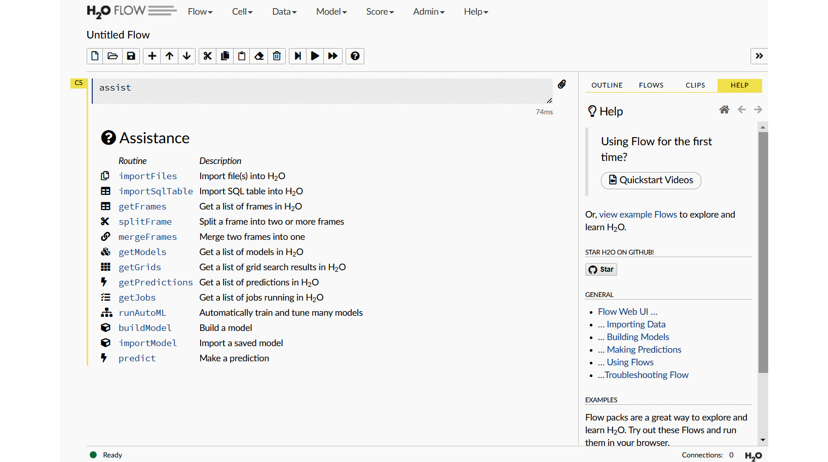
Figure 2.1 – The main page of the H2O Flow UI
Don’t be alarmed if you see something slightly different. This might be because the version you installed might be different from the one shown in this book. Nevertheless, the basic setup of the UI should be similar. As you can see, there are plenty of interactive options to choose from. This can be a little overwhelming at first, so let’s take it piece by piece.
At the very top of the web page, there are various ML object operations, each with its own drop-down list of functions. They are as follows:
- Flow: This section contains all operations related to the Flow notebook.
- Cell: This section contains all operations related to the individual cells in the notebook.
- Data: This section contains all operations related to data manipulations.
- Model: This section contains all operations related to model training and algorithms.
- Score: This section contains all operations related to scoring and making predictions.
- Admin: This section contains all administrative operations such as downloading logs.
- Help: This section contains all links to H2O documentation for additional details.
We will go through them in greater detail, step by step, once we start creating our ML pipeline later.
The following screenshot shows you the various ML function operations of the H2O Flow UI:

Figure 2.2 – The ML object operation toolbar
Following this, we have the Flow Name and Flow Toolbar settings. By default, the flow name will be Untitled Flow. The flow name helps identify the whole flow in general so that you do not mix the different experiments. The Flow Toolbar section is a simple toolbar that helps you with basic operations such as editing and managing the cells in your flow.
The following screenshot shows you the flow toolbar that is present on the main page:
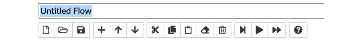
Figure 2.3 – The Flow Name and flow toolbar sections
Cells are lines of code executions that you can perform one by one. They can also be used to make comments, headings, and even Markdown text.
The tools are listed as follows. We will start from left to right:
- New: This creates a new Flow notebook.
- Open: This opens an existing Flow notebook that is stored in your system.
- Save: This saves your current flow.
- Insert Cell: This inserts a cell below.
- Move up: This moves the currently highlighted cell up over the above cell.
- Move down: This moves the currently highlighted cell to below the cell under it.
- Cut: This cuts the cell and stores it on the clipboard.
- Copy: This copies the currently highlighted cell.
- Paste: This pastes the previously copied cell below the currently highlighted cell.
- Clear Cell: This clears the output of the cell if there is any.
- Delete Cell: This deletes the cell entirely.
- Run and Select below: This runs the currently highlighted cell and stops at the cell below.
- Run: This runs the currently highlighted cell.
- Run all: This runs all the cells from top to bottom one by one.
- Assist me: This executes an assist command that helps you by showing links to basic ML commands.
On the right-hand side of your flow are additional support options to help you manage your workflow. You have OUTLINE, FLOW, CLIPS, and HELP. Each option has its own column with functional details.
The following screenshot shows you the various support options of the H2O Flow UI:

Figure 2.4 – Support options
The OUTLINE column shows you a list of all the executions you performed. Looking at the outline helps you to quickly check whether all the steps you performed when creating your ML pipeline were in the correct sequence, whether there were any duplicates, or whether any incorrect steps were made.
The following screenshot shows you the OUTLINE support option section:
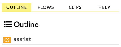
Figure 2.5 – OUTLINE
The FLOW column shows you all your previously saved flows. At the moment, you won’t have any, but once you do save a flow, it will show up here with a quick link to open it. Please note that only one Flow notebook can be opened at a time on the H2O Flow page. If you want to work on multiple flows simultaneously, you can do so by opening another tab and opening the Flow notebook there.
The following screenshot shows you the FLOWS support option section:
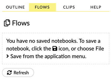
Figure 2.6 – Saved flows
The CLIPS column is your clipboard. If there is any code to be executed that you will be running multiple times in your flow, then you can write it once and save it to your clipboard by selecting the paper clip icon on the right-hand side of your cell. Then, you can paste that cell whenever you need it again without needing to search for it in your flow. The clipboard also stores a set number of trash cells.
The following screenshot shows you the CLIPS support option section:
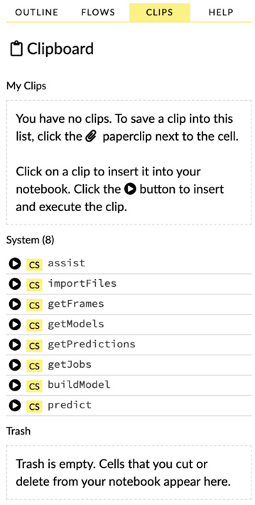
Figure 2.7 – Clipboard
The HELP column shows you various resources to help the user use H2O Flow. This involves QuickStart videos, example flows, general usage examples, and links to the official documentation. Feel free to explore these to gain an understanding of how you can use H2O Flow.
The following screenshot shows you the Help support option section:
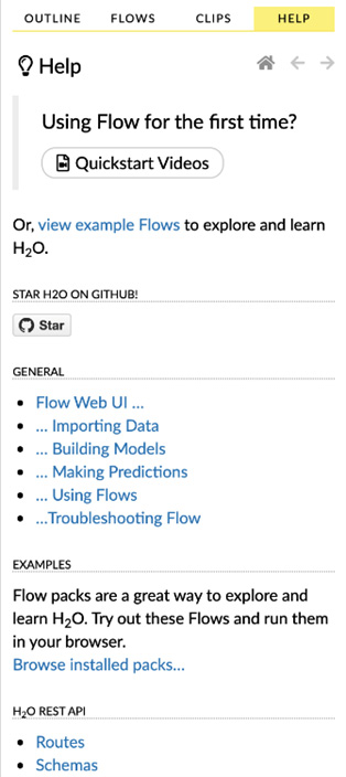
Figure 2.8 – The Help section
Back to the top of the page, let’s explore the first two drop-down lists. They are simple enough to understand.
The following screenshot shows you the first drop-down list of operations, that is, the Flow object operations:
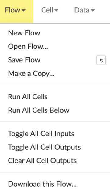
Figure 2.9 – The Flow functions drop-down list
The Flow drop-down list of operations has basic functionality in terms of the Flow notebook in general. You can create a new flow, open an existing one, save, copy, run all of the cells in the flow, clear the outputs, and download flows. Downloading flows is very useful, as you can easily transfer your ML work from the flows to other systems.
On the right-hand side is the Cell object operation drop-down list (as shown in Figure 2.10). This drop-down list is also simple to understand. It has basic functionality to manipulate the various cells in the flow. Usually, it targets the highlighted cell in the Flow notebook. You can change the highlighted cell by just clicking on it:
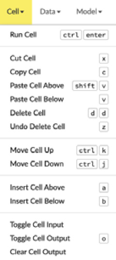
Figure 2.10 – The Cell functions drop-down list
We will explore the other options as we start working on our ML pipeline.
In this section, we understood what H2O Flow is, how to download it, and how to launch it locally. Additionally, we explored the various parts of the H2O Flow UI and the various functionalities it has to offer. Now that we are familiar with our environment, let’s dive in deeper and create our ML pipeline. We will start with the very first part of the pipeline, that is, handling data.
Working with data functions in H2O Flow
An ML pipeline always starts with data. The amount of data you collect and the quality of that data play a very crucial role when training models of the highest quality. If one part of the data has no relationship with another part of the data, or if there is a lot of noisy data that does not contribute to the said relationship, the quality of the model will degrade accordingly. Therefore, before training any models, often, we perform several processes on the data before sending it to model training. H2O Flow provides interfaces for all of these processes in its Data operation drop-down list.
We will understand the various data operations and what the output looks like in a step-by-step process as we build our ML pipeline using H2O Flow.
So, let’s begin creating our ML pipeline by, first, importing a dataset.
Importing the dataset
The dataset we will be working with in this chapter will be the Heart Failure Prediction dataset. You can find the details of the Heart Failure Prediction dataset at https://www.kaggle.com/fedesoriano/heart-failure-prediction.
This is a dataset that contains certain health information about individuals with cholesterol, maximum heart rate, chest pain, and other attributes that are important indicators of whether a person is likely to experience heart failure or not.
Let’s understand the contents of the dataset:
- Age: The age of the patient in years
- Sex: The sex of the patient; M for male and F for female
- ChestPainType:
- The types are listed as follows:
- TA: Typical Angina
- ATA: Atypical Angina
- NAP: Non-Anginal Pain
- ASY: Asymptomatic
- The types are listed as follows:
- RestingBP: Resting blood pressure in [mm Hg]
- Cholesterol: Serum cholesterol in [mm/dl]
- FastingBS: Fasting blood sugar, where it is 1 if FastingBS is greater than 120 mg/dl, else it is 0
- RestingECG: Resting electrocardiogram results
- The types are listed as follows:
- Normal: Normal
- ST: Having ST-T wave abnormality
- LVH: Showing probable or definite left ventricular hypertrophy by Estes’ criteria
- The types are listed as follows:
- MaxHR: The maximum heart rate achieved value, lying between 60 and 202
- ExerciseAngina: Exercise-induced angina; Y for yes, and N for no
- Oldpeak: ST (Numeric value measured in depression)
- ST_Slope: The slope of the peak exercise ST segment
- The types are as follows:
- Up: Sloping upward
- Flat: Flat
- Down: Sloping downward
- The types are as follows:
- HeartDisease: The output class, where 1 indicates heart disease and 0 indicates no heart disease
We will train a model that tries to predict whether a person with certain attributes has the potential to face heart failure or not by using this dataset. Perform the following steps:
- First, let’s start by importing this dataset using H2O Flow.
- On the topmost part of the web UI, you can see the Data object operations drop-down list.
- Click on it, and the web UI should display an output that looks like the following screenshot:
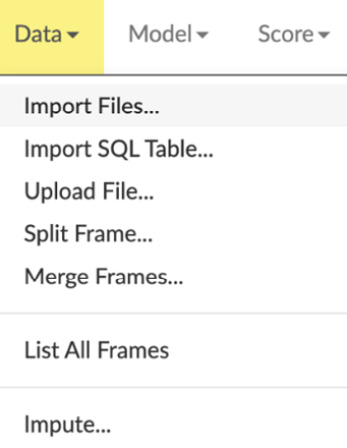
Figure 2.11 – The Data object drop-down list
The drop-down list shows you a list of all the various operations that you can perform, along with those that are related to the data you will be working with.
The functions are listed as follows:
- Import Files: This operation imports files stored in your system. They can be any readable files edited in Comma-Separated Values (CSV) format or Excel format.
- Import SQL Table: This operation lets you import the data stored in your Structured Query Language (SQL) table if you are using an SQL database to store any tabular data. When you click on it, you will be prompted to input the Connection URL value to your SQL database, along with its credentials, the Table name, the Columns name, and an option to select Fetch mode, which could be DISTRIBUTED or SINGLE, as shown in the following screenshot:
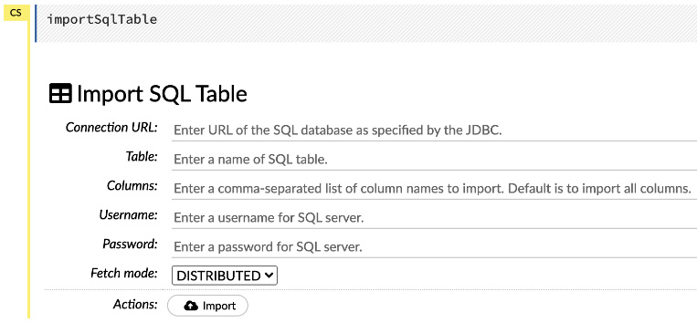
Figure 2.12 – Import SQL Table
- Upload File: This operation uploads a single file from your system and parses it immediately.
- Split Frame: This operation splits the dataframe that has already been imported and parsed by H2O Flow into multiple frames, which you can use for multiple experiments.
- Merge Frames: This operation merges multiple frames into one. When you click on it, you will be prompted to select the right and left frames and their respective columns. Additionally, you have the flexibility to select which rows from which frame to include in the merge, as shown in the following screenshot:
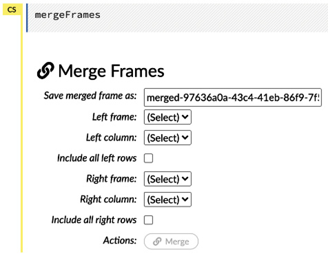
Figure 2.13 – Merge Frames
- List frames: This operation lists all the frames that are currently imported and parsed by H2O. This helps if you want to run your pipeline on different datasets that were previously imported or stitched by you.
- Impute: Imputation is the process of replacing a missing value in the dataset with an average value such that it does not introduce any bias with a minimized value, a maximized value, or even an empty value. This operation lets you replace these values in your frame depending on your preference.
So, first, let’s import the Heart Failure Prediction dataset.
- Click on the Data operation drop-down list.
- Click on Import Files…. You should see an operation executed on a cell in your flow, as shown in the following screenshot:
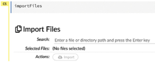
Figure 2.14 – Import Files
You can also directly run the same command by typing importFiles into a cell and pressing Shift + Enter instead of using the drop-down list.
- In the search bar, add the location of the folder in which you have downloaded the dataset.
- Click on the search button on the extreme right-hand side. This will show you all the files in the folder, and you can select which ones to import.
- Select the heart.csv dataset, as shown in the following screenshot:
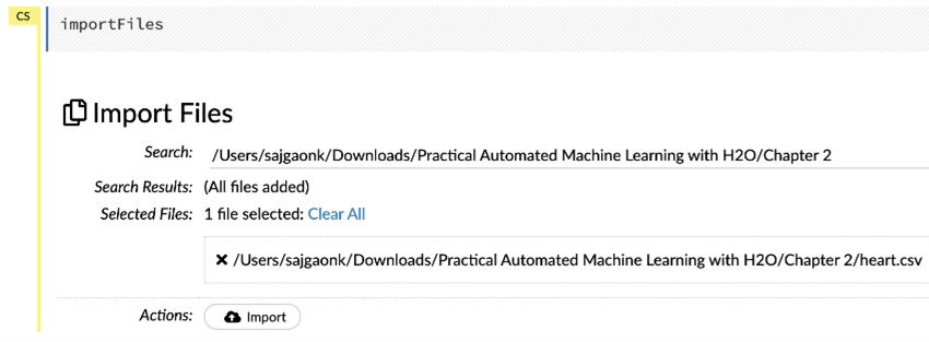
Figure 2.15 – Importing files with inputs
- Once you have selected the file, click on the Import button. H2O will then import the dataset and show you an output, as follows:
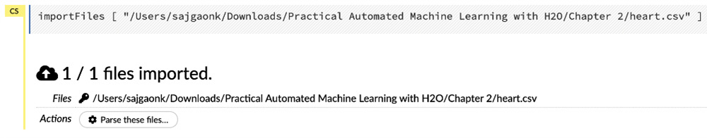
Figure 2.16 – The imported files
Congratulations! You have now successfully imported your dataset into H2O Flow. The next step is to parse it into a logical format. Let’s understand what parsing and is how we can do it in H2O Flow.
Parsing the dataset
Parsing is the process of analyzing the string of information in a dataset and loading it into a logical format, in this case, a hex file. A hex file is a file whose contents are stored in a hexadecimal format. H2O uses this file type internally for dataframe manipulations and maintains the metadata of the dataset.
Let’s parse the newly imported dataset by executing the following steps:
- Click on the Parse these files… button after importing the dataset, as shown in Figure 2.16.
The following screenshot shows the output you should expect:
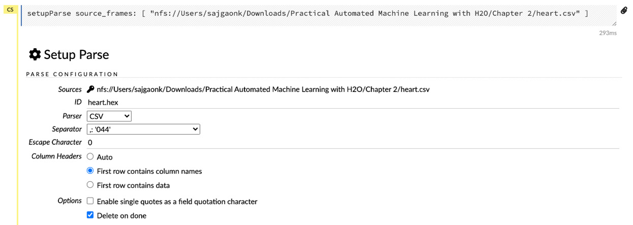
Figure 2.17 – The dataset parsing inputs
- Then, you will be prompted to input the PARSE CONFIFUGRATION settings to parse the dataset. H2O will read the dataset using these configurations and create a hex file. During parsing, you have the following configurations to select from:
- Sources: This configuration denotes the source of the dataset you will be parsing.
- ID: This configuration indicates the ID of the dataset. You can change the ID of the hex file that will be created.
- Parser: This configuration sets the parser to use for parsing your dataset. You will be using different parsers to parse different types of datasets. For example, if you are parsing a Parquet file, then you will need to select the Parquet file parser. In our case, we are parsing a CSV file; hence, select the CSV parser. You can set it to AUTO too, and H2O will self-identify which parser will be needed to parse the specified file.
- Separator: This configuration is used to specify the separator that separates the values in the dataset. Let’s leave it at the default value, ,:’004’, which is a very commonly found CSV separator value.
- Escape Character: This configuration is used to specify the escape character that is used in the dataset. Let’s leave it at the default value.
- Column Headers: This configuration is used to specify whether the first row of the dataset contains column names or not. H2O will use this information to handle the first row to either use it as column information or autogenerate column names and use the first row as data values. Additionally, you can set the value to Auto to let H2O self-identify whether the first row of the dataset contains column names or not. Our dataset has the first row as column names, so let’s select First row contains column names.
- Options: This configuration contains additional operations as follows:
- Enable single quotes as a field quotation character: This option enables single quotes as a field quotation character.
- Delete on done: This option deletes the imported dataset once it has been successfully parsed. Let’s tick mark this option, as we won’t be needing the imported dataset once we successfully parse it.
- Below the PARSE CONFIGURATION section, you have the Edit Column names and Types section (see Figure 2.18). Before parsing the dataset, H2O reads the dataset and shows you a brief summary of the column names and the types of information they extracted. This gives you the option of editing your column names and types in case it has interpreted something incorrectly or if you wish to change the column names to something different.
The following screenshot shows you the column names and the option to edit their type when parsing the dataset:
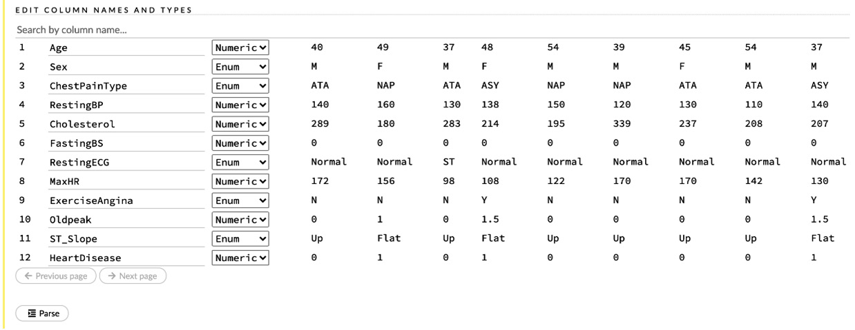
Figure 2.18 – Editing the column types
Now, let’s briefly understand the types of the columns, as shown in the preceding screenshot:
They can be listed as follows:
- Numeric: This indicates that the values in the column are numbers.
- Enum: This indicates that the values in the column are Enumerated Types (Enums). Enums are a certain set of named values that are non-numeric and finite in nature.
- Time: This indicates that the values in the column are datetime data type values.
- UUID: This indicates that the values in the column are Universally Unique Identifiers (UUIDs).
- String: This indicates that the values in the column are string values.
- Invalid: This indicates that the values in the column are invalid, which means that there are some issues with the values in the column.
- Unknown: This indicates that the values in the column are unknown, which means that the column contains no values.
During training, H2O treats the columns of the dataframe differently depending on their type. Sometimes, it misinterprets the values of the columns and assigns an incorrect column type to a column. Take a look at the columns of the datasets and their corresponding types. You might notice that after importing the dataset, the type of our HeartDisease output column is Numeric. H2O read the 1 and 0 and assumed its type was Numeric. But it is, in fact, an Enum value, as 1 indicates heart disease, and 0 indicates no heart disease. There is no numerical value in between. We always need to be careful when parsing datasets. We need to ensure that H2O interprets the dataset correctly before we start training models on it. H2O Flow provides an easy way to correct this before parsing.
Next, let’s correct the column types:
- Select the drop-down list next to the HeartDisease column name and set it to Enum.
- Similarly, FastingBS will be set as Numeric, but it is, in fact, an Enum value based on its description. So, let’s set it to Enum.
- Now that we have corrected the column types and have selected the correct parsing configurations, let’s parse the dataset. Click on the Parse button at the bottom of the output.
The following screenshot shows you the output after parsing:
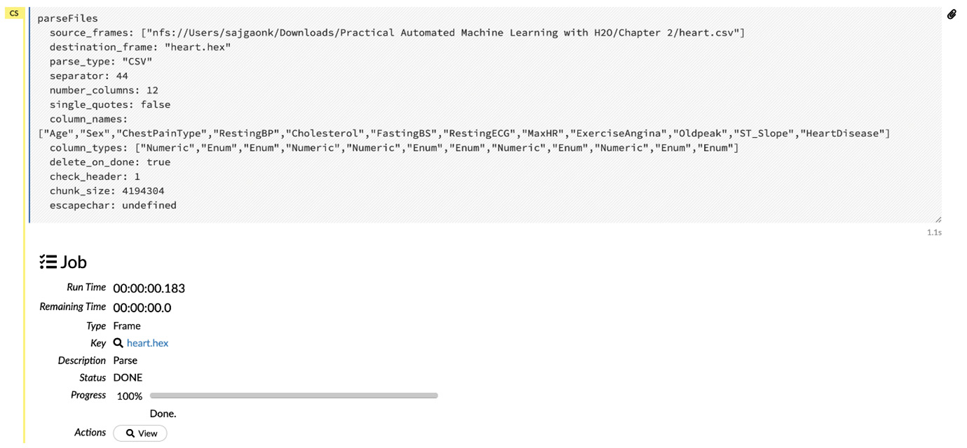
Figure 2.19 – Parsing the output
Now, let’s observe the output we got from the preceding screenshot:
- Run Time: This output shows you the runtime since H2O started to parse the dataset.
- Remaining Time: This output shows you the expected remaining time it will take H2O to finish parsing the dataset.
- Type: This output shows you the parsed file’s type.
- Key: This output shows you a link to the hex file, which has been generated after successfully parsing.
- Description: This output shows you the operation currently being performed.
- Status: This output shows you the current status of the operation.
- Progress: This output shows you the progress bar of the operation.
- Action: This output is a button that shows you the hex file that has been generated after successfully parsing the dataset.
Congratulations! You have successfully parsed your dataset and have generated the hex file. The hex file is commonly termed a dataframe. Now that we have a dataframe generated, let’s see the various metadata and operations available to us to be performed on the dataframe.
Observing the dataframe
The dataframe is the primary data object on which H2O can perform several data operations. Additionally, H2O provides detailed insights and statistics on the contents of the dataframe. These insights are especially helpful when working with very large dataframes, as it is very difficult to identify whether there are any missing or zeros in any of the columns where data rows can span from thousands to millions.
So, let’s observe the dataframe we just parsed and explore its features. You can view the dataframe by performing either of the following actions from the parsing output that we saw in Figure 2.19:
- Click on the heart.hex hyperlink in the Key row.
- Click on the View Data button in the Actions row.
The following screenshot shows you the output of the previously mentioned actions:
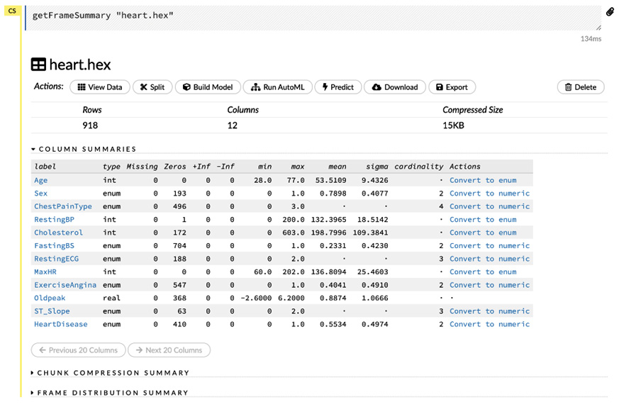
Figure 2.20 – Viewing a dataframe
The output displays a summary of the dataframe. Before exploring the various operations in the Actions section, first, let’s explore the metadata of the dataframe that is shown below it.
The metadata consists of the following:
- Rows: Displays the number of rows in the dataset
- Columns: Displays the number of columns in the dataset
- Compressed Size: Displays the total compressed size of the dataframe
Below the metadata, you have the COLUMN SUMMARIES section. Here, you can see statistics about the contents of the dataframe split across the columns.
The summary contains the following information:
- label: This column shows the name of the columns of the dataframe.
- type: This column shows the type of the column.
- Missing: This column shows the number of missing values in that column.
- Zeros: This column shows the number of zeros in the column.
- +Inf: This column shows the number of positive infinity values.
- -Inf: This column shows the number of negative infinity values.
- min: This column shows the minimum value in the column.
- max: This shows the maximum value in the column.
- sigma: This column shows the variability in the values of the column.
- cardinality: This column shows the number of unique values in the column.
- Actions: This column shows certain actions that you can perform on the columns of the dataframe. These actions mostly consist of converting the columns into different types. It is useful in correcting the column types if they were read incorrectly by H2O after parsing.
You might be wondering why you are seeing plenty of values in the Zeros columns for columns such as Sex and RestingECG. This is because of encoding. When parsing enum columns, H2O encodes enums and strings into numerical values starting from 0 to 1, then 2, and so on and so forth. You can also control this encoding process by selecting which encoding process you want, for example, Label encoding or One-hot encoding. We will discuss encoding in greater detail in Chapter 5, Understanding AutoML Algorithms.
After the COLUMN SUMMARIES section, you will see the CHUNK COMPRESSION SUMMARY section, as shown in the following screenshot:
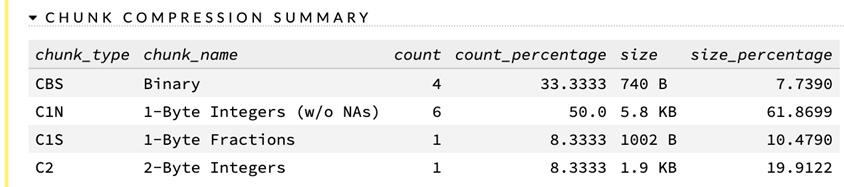
Figure 2.21 – The dataset’s CHUNK COMPRESSION SUMMARY section
When working with very large datasets, it can take a very long time to read and write data from the datasets if done in a traditional manner. Therefore, systems such as Hadoop File System, Spark, and more are often used as they perform read and write in a distributed manner, which is faster than the traditional contiguous manner. Chunking is a process where distributed file systems such as Hadoop split the dataset into chunks and flatten them before writing to disk. H2O handles all of this internally so that users do not need to worry about managing distributed read or write. The CHUNK COMPRESSION SUMMARY section just gives additional information about the chunk distribution.
Underneath CHUNK COMPRESSION SUMMARY is the FRAME DISTRIBUTION SUMMARY section, as shown in the following screenshot:
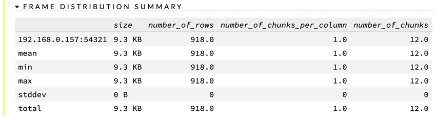
Figure 2.22 – The dataset’s Frame Distribution Summary section
The FRAME DISTRIBUTION SUMMARY section gives statistical information about the dataframe in general. If you have imported multiple files and parsed them into a single dataframe, then the frame distribution summary will calculate the total size, the mean size, the minimum size, the maximum size, the number of chunks per dataset, and more.
Looking back at the dataframe from Figure 2.20, you can see that the column names are highlighted as links. Let’s click on the last column, HeartDisease.
The following screenshot will show you a column summary of the HeartDisease column:
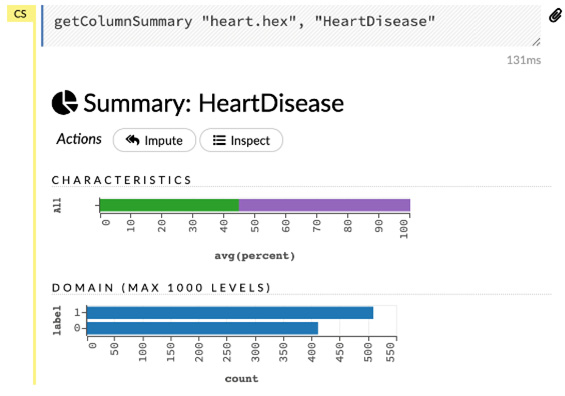
Figure 2.23 – Column summary
The Column Summary gives you more details about individual columns in the dataset based on their type.
For enums such as HeartDisease, it shows you the details of the column as follows:
- Characteristics: This graph shows you the percentage distribution of zero and nonzero values.
- Domain: This graph shows you the domain of the column, that is, the number of times a value has been repeated over the total number of rows.
You will see more details when you hover your mouse over the graphs. Feel free to explore all the columns and try to understand their features.
Returning to the dataframe from Figure 2.20, let’s now look at the Actions section. This includes certain actions that are available to be performed on the dataframe.
Those actions include the following:
- View Data: This action displays the data in the dataframe.
- Split: This action splits the dataframe into the specified parts in the specified ratio.
- Build Model: This action starts building a model on this dataframe.
- Run AutoML: This action triggers AutoML on the dataframe.
- Predict: This action uses the dataframe to predict on an already trained model and gets results.
- Download: This action downloads the dataframe to the system.
- Export: This action exports the dataframe to a specified path in the system.
As much as we are excited to trigger AutoML, let’s continue our exploration of the various dataframe features.
Now, let’s see the dataframe and its actual data contents. To do this, click on the View Data button in the Actions section.
The following screenshot shows you the output of the View Data button:
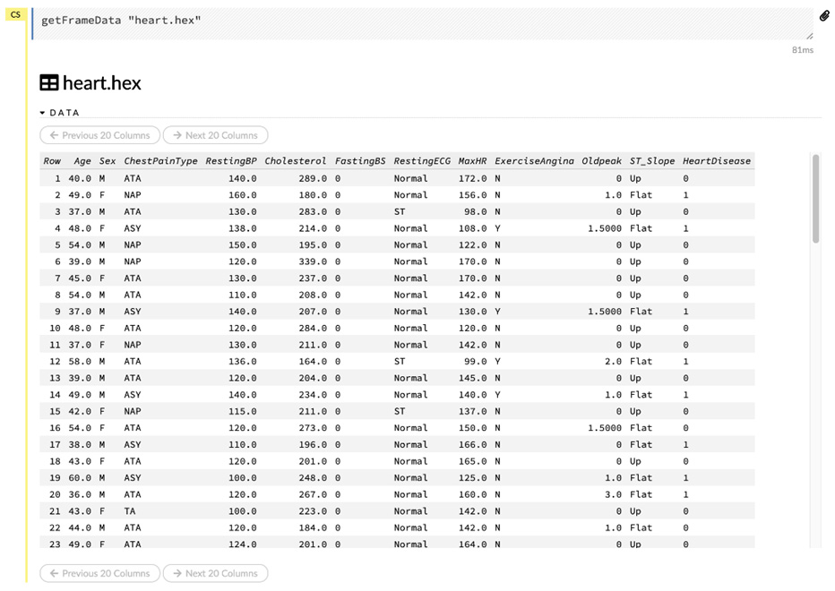
Figure 2.24 – The dataframe’s content view
This function shows the actual contents of the dataset. You can scroll down to see all of the contents of the dataframe. If you have run any operations on the dataframe, then you will be able to view the changes in the content of the dataframe using this operation.
Now that you have explored and understood the various dataframe operations and metadata of the dataframe, let’s investigate another interesting dataframe operation called Split.
Splitting a dataframe
Before we send a dataframe for model training, we need a sample dataframe with predicted values. This sample can be used to validate whether the model is making a correct prediction or not and measure the accuracy and performance of the model. We can do this by reserving a small part of the dataframe to be used later for validation. This is where split functionality comes into the picture.
Split, as the name suggests, splits the dataset into parts that we can later use for different operations. Splitting of dataset takes ratios into account. H2O creates multiple dataframes based on the number of splits you want to make and the ratio of the distribution of data.
To split the dataframe, click on the Split operation button in the Actions section.
The following screenshot shows you the output of clicking on the Split button:
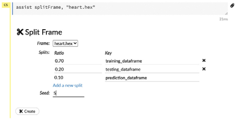
Figure 2.25 – Splitting a dataframe
In the preceding output, you will be prompted to input the splitting configurations, which are listed as follows:
- Frame: This configuration lets you select the frame that you want to split.
- Splits: This configuration lets you select the number of splits that you want to make and the ratio of the distribution of data you want among them. Additionally, you can set the key names for the splits. For our walk-through, let’s split the dataframe into three dataframes:
- training_dataframe with a ratio of 0.70
- validation_dataframe with a ratio of 0.20
- testing_dataframe with a ratio of 0.10
- Seed: This configuration lets you select the randomization point. Split does not split the dataframe linearly. It splits the rows of the dataframe randomly. This is a good thing, as it equally distributes the data between the split dataframes, thus removing any bias that might be present in the sequence of the dataset rows. For our walk-through, let’s set the seed value to 5.
Once you have made these changes, click on the Create button. This will generate three dataframes: training_dataframe, validation_dataframe, and testing_dataframe. These three frames will be stored in H2O’s local repository and can be available for other experiments, too.
The following diagram shows you the output of the Create operation:
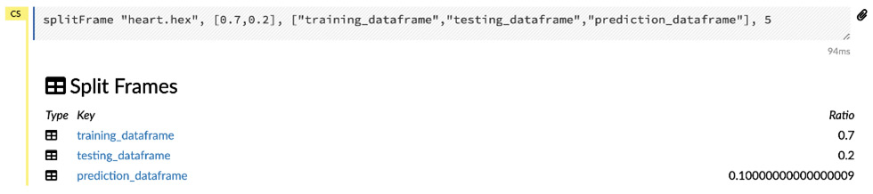
Figure 2.26 – Split dataset results
All three of the dataframes are independent dataframes and have the same set of features and options as you saw for the original dataset in Figure 2.20. Splitting does not delete the original dataframe. It creates new dataframes and copies the data from the original dataframe and distributes them among the dataframes based on the selected ratios.
Now that we have the training frame, the validation frame, and the testing frame ready, we are ready for the next step of the model training pipeline, that is, model training.
So, to recap, in this section, you understood the various data operations we can perform on the dataset available in H2O Flow such as importing, parsing, reading the parsed dataframe, and splitting it.
In the next section, we will focus on model training and using H2O AutoML to train models on the dataframes we created in this heading.
Working with model training functions in H2O Flow
Once your dataset is ready, the next step of the model training pipeline is the actual training part. The training of models can get very complex as there are a lot of configurations that decide how the model will be trained on the dataset. This is true even for AutoML where the majority of the hyperparameter tuning is done behind the scenes. Not only are there right and wrong ways of training a model for a specific type of data, but some of the configuration values can also affect the performance of the model. Therefore, it is important to understand the various configuration parameters that H2O has to offer when training a model using AutoML. In this section, we will focus on understanding what these parameters are and what they do when it comes to model training.
We will understand how to train a model using AutoML, step by step, using the dataframes we created previously.
Note that there are plenty of things in this section that will be too complex to understand at this stage. We will explore some of them in future chapters. For the time being, we will only focus on features we can understand right now, as the goal of this chapter is to understand H2O Flow and how to use AutoML to train models using H2O Flow.
In the following sub-sections, we will gain an understanding of the model training operations, starting with an understanding of the AutoML training configuration parameters.
Understanding the AutoML parameters in H2O Flow
H2O AutoML is extremely configurable in terms of how you want to train your models. Despite using the same AutoML technology, often, every industry will have certain preferences or inclinations regarding how it wants to train its models based on their requirements. So, even though AutoML is automating most of the ML processes, a degree of control and flexibility is still needed in terms of how AutoML trains its models. H2O provides extensive configuration capabilities for its AutoML feature. Let’s explore them as we train our model.
There are two ways that you can trigger AutoML on a dataset. They are listed as follows:
- By clicking on the Run AutoML button in the Actions section of your dataframe output, as shown in Figure 2.20.
- By selecting Run AutoML in the drop-down menu of the Model section, on the topmost part of the web UI, as shown in Figure 2.27.
Let’s go with the second option so that we can explore the Model operations section at the top of the web UI page. When you click on the Model section, you should see the drop-down list, as shown in the following screenshot:
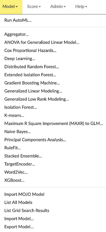
Figure 2.27 – The Model functions drop-down list
The preceding drop-down list categorizes the model operations into three types, as follows:
- Run AutoML: This operation starts the AutoML process by prompting the user to input configuration values to train models using AutoML.
- Run Specific Models: This operation starts model training on specific ML algorithms that you wish to use; for example, deep learning, K-means clustering, random forest, and more. Each ML algorithm comes with its own set of parameters that you must specify to start training models.
- Model Management options: These operations are basic operations that are used to manage the various models you might have trained over a period of time.
- The operations are listed as follows:
- Import MOJO Model: This operation imports H2O Model Object, Optimized (MOJO) models previously trained by another H2O service and exported to the system in the form of a MOJO.
- List All Models: This operation lists all the models trained by your H2O service. This includes those trained by other Flow notebooks.
- List Grid Search Results: Grid search is a technique that is used to find the best hyperparameters when training a model to get the best and most accurate performance out of it. This operation lists all the grid search results from the model training.
- Import Model: This operation imports model objects into H2O.
- Export Model: This operation exports model objects to the system either as a binary file or as a MOJO.
- The operations are listed as follows:
Now, let’s use AutoML to train our model on our dataset.
Click on Run AutoML. As shown in Figure 2.27, you should see an output prompting you to input a wide variety of configuration parameters to run AutoML. There are tons of options to configure your AutoML training. These can greatly affect your model training performance and the quality of the models that eventually get trained. The parameters are classified into three categories. Let’s explore them, one by one, categorically and input the values to suit our model training requirements starting with the basic parameters.
Basic parameters
Basic parameters are parameters that focus on the basic inputs needed for all model training operations. These are common among all the ML algorithms and are self-explanatory.
The following screenshot shows you the basic parameter values you need to input to configure AutoML:
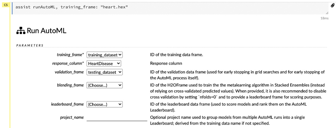
Figure 2.28 – The basic parameters of AutoML
The basic parameters are listed as follows:
- training_frame: This configuration sets the dataframe to be used for training the model and is mandatory. In our case, our training_frame parameter is the training_dataframe.hex file that we created in the Working with data functions in H2O Flow section.
- response_column: This configuration sets the response column of the dataframe that is to be predicted. This is a mandatory parameter. In our case, our response column is the HeartDisease column.
- validation_frame: This configuration sets the dataframe to be used for validation of the model during training. In our case, our validation frame is the validation_dataframe.hex file we created in the previous section.
- blending_frame: This configuration sets the dataframe that should be used to train the stacked ensemble models. For the time being, we can ignore this as we won’t be exploring stacked ensemble very much in this chapter. We will explore stacked ensemble models in more detail in Chapter 5, Understanding AutoML Algorithms, so let’s leave this blank.
- leaderboard_frame: This configuration sets the ID of the dataframe, which will be used to calculate the performance metrics of the trained models, and it will use the results to rank them on the leaderboard. If a leaderboard frame has not been specified, then AutoML will use cross-validation metrics to rank the models. Even if cross-validation is turned off by setting nfolds to 0, then AutoML will generate a leaderboard from the training frame.
- project_name: This configuration sets the name of your project. AutoML will group all of the results from multiple runs into a single leaderboard under this project name. If you leave this value blank, H2O will autogenerate a random name for the project on its own.
- distribution: This configuration is used to specify the type of distribution function to be used by ML algorithms. Algorithms that support the specified type of distribution function will use it, while others will use their default value. We will learn more about distribution functions in Chapter 5, Understanding AutoML Algorithms.
Now that you understood what the basic parameters of AutoML are, let’s gain an understanding of the advanced parameters.
Advanced parameters
Advanced parameters provide additional configurations for training models using AutoML. These parameters have certain default values set to them and, therefore, are not mandatory. However, they do provide additional configurations that change the behavior of AutoML when training models.
The following screenshots show you the first part of the advanced parameters for AutoML:
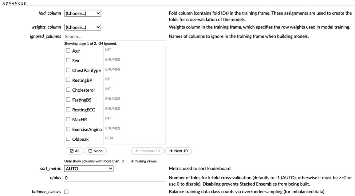
Figure 2.29 – AutoML advanced parameters, part 1
Immediately below this will be the second part of the advanced parameters. Scroll down to see the remaining parameters, as shown in the following screenshot:
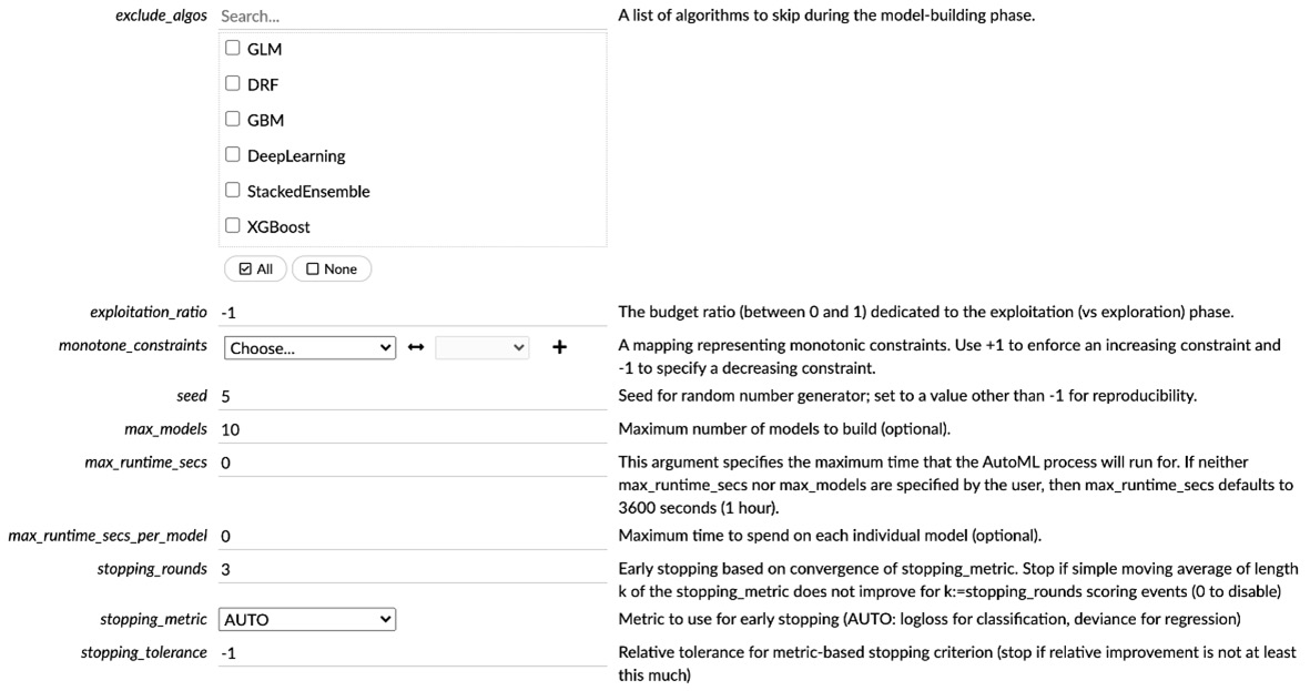
Figure 2.30 – AutoML advanced parameters, part 2
Let’s explore the parameters one by one. The advanced parameters are listed as follows:
- fold_column: This parameter uses the column values as a basis to create its folds in N-Fold cross-validation. We will learn more about cross-validation in the upcoming chapters.
- weights_column: This parameter gives weight to a column in the training frame or, put simply, gives preference to a column. We will explore weights in model training in greater detail in later chapters.
- ignored_columns: This parameter lets you select the columns from the training frame that you wish to ignore when training models. We won’t be ignoring any columns for our experiment, so we will leave all the columns unchecked.
- sort_metrics: This parameter selects the metric that will be used to sort and rank the models trained by AutoML. Selecting AUTO will use the AUC metrics for binary classification, mean_per_class_error for multinomial classification, and deviance for regression. For simplicity’s sake, let’s set Mean Squared Error (MSE) as the sorting metric since it is easier to understand. We will explore metrics in greater detail in Chapter 6, Understanding H2O AutoML Leaderboard and Other Performance Metrics.
- nfolds: This parameter selects the number of cross-validation folds created for cross-validation. Cross-validation generates stacked ensemble models. For the moment, we will set this value to 0 to prevent the creation of stacked ensemble models. We will explore stacked ensemble models and cross-validation further in the upcoming chapters.
- Balance_classes: In model training, it is always best to train models on datasets that have output classes with an equal distribution of values. This mitigates any biases that might arise from an unequal distribution of values. This parameter balances the output classes to be of equal numbers. In our case, the output class is the Heart Disease column. As we saw in the column summary of the Heart Disease column, in the distribution section, we had around 410 values as 0 and 508 values as 1 (see Figure 2.23). So, ideally, we need to balance out the classes before training a model. However, to keep things simple for the moment, we will skip the balancing of the classes and focus on understanding the basics. We will explore class balancing further in the upcoming chapters.
- exclude_algos: This parameter excludes certain algorithms from the AutoML training. For our experiment, we want to consider all the algorithms, so let’s leave the value empty.
- exploitation_ratio: This is an experimental option that sets the exploitation versus exploration ratio when training a model. We will discuss this in greater detail in the upcoming chapters. Let’s keep the default value of -1 as it is.
- monotone_constraints: In some cases, where there is a very strong prior belief that the relationship between features has some quality, constraints can be used to improve the predictive performance of the model. This parameter helps set these constraints. We will discuss this more in the upcoming chapters. Let’s leave this value empty.
- seed: This parameter sets the seed value for randomization, which is useful for reproducing results. Let’s set this to 5.
- max_models: This parameter sets the maximum number of models to be trained by H2O AutoML. We will set this to 10, else model training can take a long time.
- max_runtime_secs: This parameter sets the maximum time that H20 should spend training a single model. Usually, the larger the size of the dataset, the more time it takes for a model to train. Setting a very small runtime for model training will not give AutoML the time it needs to train models. Since our dataset is not very big, we will let AutoML take its time training the models, which shouldn’t be that long.
- max_runtime_sec_per_model: This parameter sets the maximum time AutoML should spend on training an individual model. Model training won’t take too long. So, let’s ignore this.
- stopping_round: This tells AutoML to stop training models after the stopping metric doesn’t improve much over the number of rounds. We want to train all the models, so we will set this value to 0 to disable it.
- stopping_metrics: This metric is used for early stopping. Since stopping is disabled, we will ignore this.
- stopping_tolerance: This refers to the relative tolerance of improvement on progressive model training expected below which AutoML should stop training models. Since stopping is disabled, we will ignore this.
Now that you have understood what the basic parameters of AutoML are, let’s check the expert parameters.
Expert parameters
Expert parameters are parameters that provide additional options that supplement the AutoML training results with additional features that help in further experimentation. These parameters are dependent on the configuration you already selected in the Advanced parameters section.
The following screenshot shows you the expert parameter options that are available for our current walk-through:
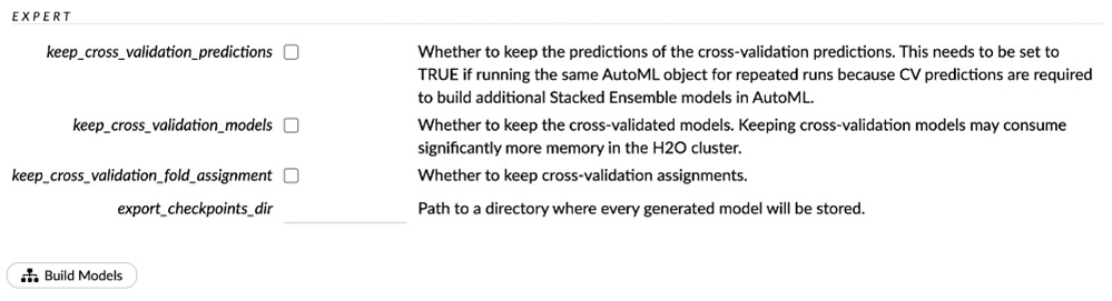
Figure 2.31 – AutoML expert parameters
The expert parameters are listed as follows:
- keep_cross_validation_predictions: If cross-validation is enabled for training, then H2O provides the option of saving those prediction values.
- keep_cross_validation_models: If cross-validation is enabled for training, then H2O provides the option of saving the models trained for the same.
- keep_cross_validation_fold_assignments: If cross-validation is enabled for training, then H2O provides the option of saving the folds used in model training for the different cross-validations.
- export_checkpoint_dir: This is the directory path where H2O will store the generated models.
More expert options become available depending on what you select in the basic and advanced parameters. For the time being, we can disable all the expert parameters as we won’t be focusing much on them in this walk-through.
Once you have set all of the parameter values, the only thing left now is to trigger the AutoML model training.
Training and understanding models using AutoML in H2O Flow
Model training is one of the most complex and important parts of the ML pipeline. Model training is the process of mapping a mathematical approximation by learning the relationship between features and the expected output, all while trying to minimize loss. There are various ways you can do this. The method by which a system performs this task is known as an ML algorithm. AutoML trains models using various ML algorithms and compares their performance with each other to find the one that has the least error metric value as per the ML problem.
First, let’s gain an understanding of how we can train a model using AutoML in H2O Flow.
Training models using AutoML in H2O Flow
You need to make careful considerations when setting the parameter values for training models using AutoML. Once you have selected the correct inputs, you can then trigger the AutoML model training.
You can do this by clicking on the Build Models button at the end of your Run AutoML output.
The following screenshot shows you the AutoML training job progress:
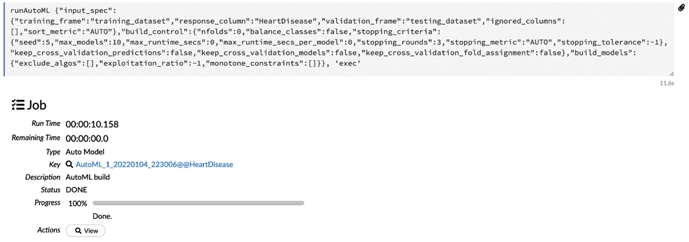
Figure 2.32 – The AutoML training is finished
It should take some time to train the models. The results of the model training are stored on a Leaderboard. The value of the Key section is a link to the leaderboard (see Figure 2.32).
You can view the leaderboard in one of two ways. They are listed as follows:
- Click on the leaderboard link in the Key section of the AutoML training job output.
- Click on the View button of the AutoML training job output.
In the following screenshot, you can see what a Leaderboard looks like:
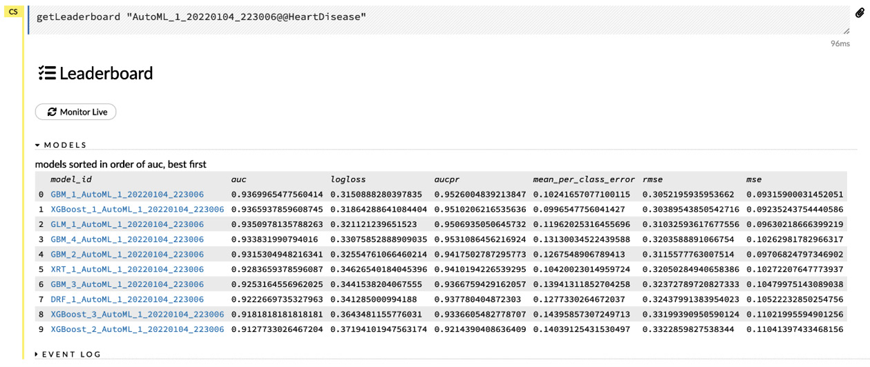
Figure 2.33 – AutoML Leaderboard
If you followed the same steps, as shown in the previous examples, then you should see the same output, albeit with slightly different IDs for the models as it is randomly generated.The leaderboard shows you all the models that AutoML has trained and ranks them from best to worst based on the sorting metric. A sorting metric is a statistical measurement of the quality of a model, which is used to compare the performance of different models. Additionally, the leaderboard has links to all the individual model details. You can click on any of them to get more information about the individual models. If AutoML is in progress and currently training models, then you can also view the progress of the training in real time by clicking on the Monitor Live button.
Now that you have understood how to train a model using AutoML, let’s dive deep into the ML model details and try to understand its various characteristics.
Understanding ML models
An ML model can be described as an object that contains a mathematical equation that can identify patterns for a given set of features and predict a potential outcome. These ML models form the central component of all ML pipelines, as the entire ML pipeline aims to create and use these models for predictions. Therefore, it is important to understand the various details of a trained ML model in order to justify whether the predictions that it is making are accurate or not and to what degree they are accurate.
Let’s click on the best model on the leaderboard to understand more of its details. You should see the following output:
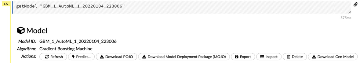
Figure 2.34 – Model information
As you can see, H2O provides a very in-depth view of the model details. All the details are categorized inside their own sub-sections. There is a lot of information here, and as such, it can be overwhelming. For the moment, we will only focus on the important parts.
Let’s glance through the important and easy-to-understand details one by one:
- Model ID: This is the ID of the model.
- Algorithm: This indicates the algorithm used to train the model.
- Actions: Once the model has been trained, you can perform the following actions on it:
- Refresh: This refreshes the model in memory.
- Predict: This lets you start making predictions on this model.
- Download POJO: This downloads the model in Plain Old Java Object (POJO) format.
- Download Model Deployment Package: This downloads the model in MOJO format.
- Export: This exports the model as either a file or MOJO to the system.
- Inspect: H2O goes into inspect mode, where it inspects the model object, retrieving detailed information about its schemas and sub-schemas.
- Delete: This deletes the model.
- Download Gen Model: This downloads the generated model JAR file.
Then, you have a set of sub-sections explaining more about the model’s metadata and performance. These sub-sections vary slightly for different models, as some models might need to show some additional metadata for explainability purposes.
As you can see, a lot of the details seem very complex in nature and they are rightfully so. This is because they involve a bit of data science knowledge. Don’t worry; we will explore all of them in the upcoming chapters.
Let’s go through the easier sub-sections so that we can understand the various metadata of the ML models:
- Model Parameters: The model parameters are nothing but the input parameters we passed to AutoML, along with some inputs AutoML decided to use to train the model. You can choose to view either all of the parameters or only the modified ones by clicking on the Show all parameters or Show modified parameters buttons. The description of the parameters is shown next to every parameter.
- Variable Importances: Variable importances denote the importance of the variable when it comes to making predictions. Variables with the most importance are the ones the ML model relies most on when making predictions. Any changes to variables of high importance can drastically affect the model prediction.
The following screenshot shows you the scaled importance of various features from the dataframe that we used to train models:
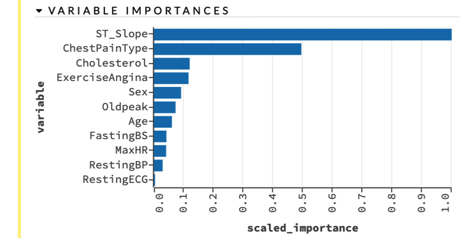
Figure 2.35 – Variable importances
- Output: The output sub-section denotes the basic output value of the AutoML training. The majority of the details that are shown are for cross-validation results.
The output values are listed as follows:
- model_category: This value indicates the category of the model that denotes what kind of prediction it performs. Binomial indicates that it performs binomial classification, which means it predicts whether the value is either 1 or 0. In our case, 1 indicates that the person is likely to face a heart condition, and 0 indicates that the person is not likely to face a heart condition.
- start_time: This value indicates the epoch time at which it started the model training.
- end_time: This value indicates the epoch time at which it ended the model training.
- run time: This value indicates the epoch total time it took to finish training the model.
- default_threshold: This is the default threshold value over which the model will consider all predictions as 1. Similarly, any value predicted below the default threshold will be 0.
The following screenshot shows you the output sub-section of the model details:
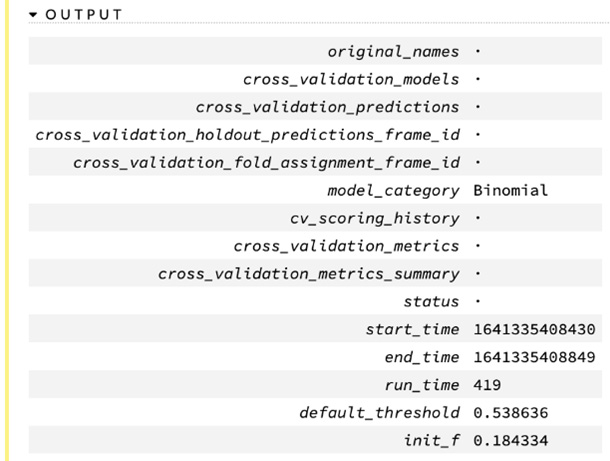
Figure 2.36 – Output of the model information
- Column_Types: This sub-section gives you a brief look at the column types of the columns in the dataframe. The values are in the same sequence as the sequence of the columns in the training dataframe.
The following screenshot shows you the column_types metrics of the model details:
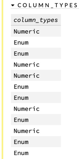
Figure 2.37 – Column types
- Output - Training_Metrics: This sub-section shows you the metrics of the model when the training dataset is used for predictions. We will learn about the various metrics of ML in future chapters.
The following screenshot shows you the training metrics of the model details:
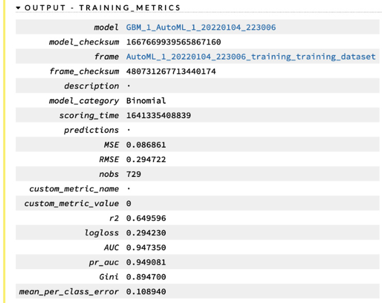
Figure 2.38 – The model output’s training metrics
- Output - Validation_Metrics: Similar to the previous sub-section, this sub-section shows you the metrics of the model when the validation dataset is used for predictions.
The following screenshot shows you the training metrics of the model details:
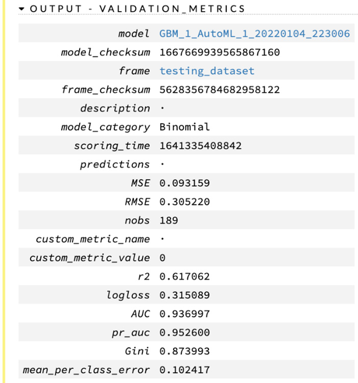
Figure 2.39 – The model output’s validation metrics
Now that we have understood the various parts of the model details, let’s see how we can perform predictions on this newly trained model.
Working with prediction functions in H2O Flow
Now that you finally have a trained model, we can perform predictions on it. Predictions on trained models are straightforward. You just need to load the model and pass in your dataset, which contains the data on which you want to make predictions. H2O will use the loaded model and make predictions for all the values in the dataset. Let’s use the prediction_dataframe.hex dataframe that we created previously to make predictions on.
We will gain an understanding of the prediction operations in the following sub-sections, starting with gaining an understanding of how to make predictions.
Making predictions using H2O Flow
First, let’s start by exploring the Score operation’s drop-down list in the topmost part of the web UI.
You will see a list of scoring operations, as follows:

Figure 2.40 – The Score functions drop-down menu
The preceding drop-down menu shows you a list of all the various scoring operations that you can perform.
The functions are listed as follows:
- Predict: This makes predictions using trained models.
- Partial Dependency Plots: These show you a graphical representation of the effects of a variable on the predictions. In other words, they show you how changing certain variables in the data used for prediction affects the prediction response.
- List all Predictions: This function lists all the predictions that were made.
There are two ways you can start making predictions in H2O Flow. They are listed as follows:
- Use the Predict function from the Score operation’s drop-down menu.
- Click on the Predict button in the Actions section of a model, as shown in Figure 2.34.
Both methods will give the same output, as shown in the following screenshot:
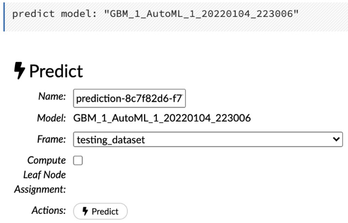
Figure 2.41 – Prediction
Clicking on the ML model’s Predict action button will set the Model parameter to the respective model ID. However, when clicking on the Predict operation button in the Scores operation drop-down list, you get the option to select any model.
The Predict operation will prompt you for the following parameters:
- Name: You can name the prediction result for easier identification. This is especially handy if you are experimenting with different prediction requests and need a quick referral to a specific prediction result of your interest.
- Model: This is the ID of the model you wish to use to make the prediction. Since we selected the Predict action of our Gradient Boosting Machine (GBM) model, this will be non-editable.
- Frame: This is the dataframe that you want to use to make predictions on. So, let’s select the prediction_dataset.hex file.
- Compute Leaf Node Assignment: This returns the leaf placements of the row in all the trees of the model for every row in the dataframe used to make the prediction. For our walk-through, we won’t need this, and as such, we can leave it unchecked.
Once you have selected the appropriate parameter values, the only thing left to do is to click on the Predict button to make your predictions.
The following screenshot shows you the output of the Predict operation:
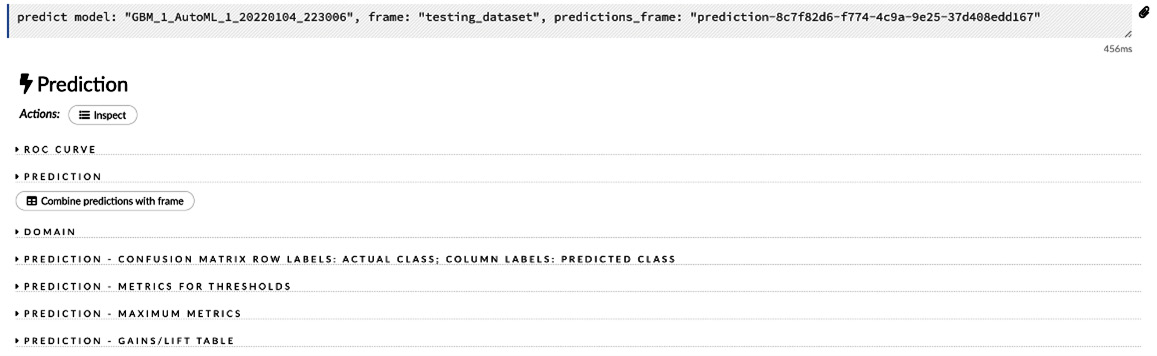
Figure 2.42 – The Prediction output
Congratulations! You have finally managed to make a prediction on a model trained by AutoML. Let’s move on to the next section, where we will explore and understand the prediction results that we just got.
Understanding the prediction results
Prediction is the final stage of the ML pipeline. It is the part that brings the actual value to all the efforts put into creating the ML pipeline. Making predictions is easy; however, it is important to understand what the actual predicted value is and what it represents against the input values.
The prediction result gives you detailed information on not only the predicted values but also metric information and certain metadata, as shown in Figure 2.42.
The following screenshot shows you the prediction output sub-section of your prediction results:
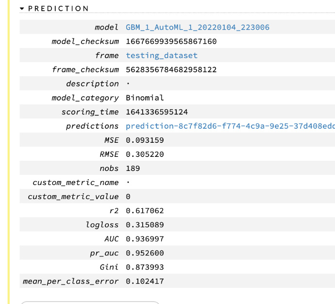
Figure 2.43 – The prediction results
This is similar to the output - validation and training metrics of the model details that we saw in Figure 2.38 and Figure 2.39.
Inside this sub-section, you have the prediction frame link next to the predictions key. Clicking on it shows you the frame summary of your prediction values. Let’s do that so that we can get a good look at the prediction values.
The following screenshot shows you the prediction summary details in the form of a dataframe:
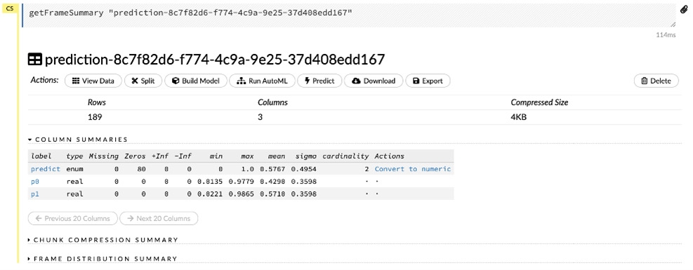
Figure 2.44 – The prediction dataframe
H2O stores prediction results as dataframes, too. Therefore, they have the same features that we discussed in the Working with Data Functions in H2O Flow section.
The COLUMN SUMMARIES section indicates the three columns in the prediction dataframe. They are listed as follows:
- Predict: This column is of the enum type and indicates the prediction value for the input rows in the prediction dataframe.
- P0: This column indicates the probability that the predicted value is 0.
- P1: This column indicates the probability that the predicted value is 1.
Let’s view the data to better understand its contents. You can view the content of the dataframe by clicking on the View Data button in the Actions section of the prediction dataframe output, as shown in Figure 2.44.
The following screenshot shows you the expected output when viewing the prediction data:
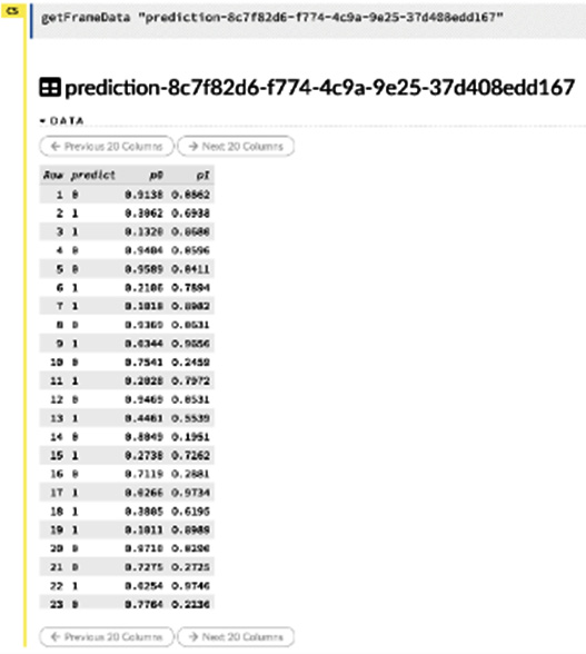
Figure 2.45 – The content of the prediction dataframe
Let’s return to the Prediction sub-section of the prediction output, as shown in Figure 2.43. Let’s combine the prediction results with the dataframe we used as input for the predictions. You can do this by clicking on the Combine predictions with frame button.
The following screenshot shows you the output of that operation:
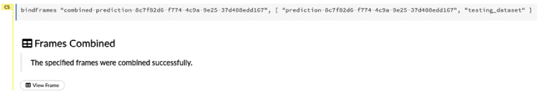
Figure 2.46 – The Combine predictions with frame result
Clicking on the View Frame button shows you the combined frame, which is also a dataframe. Let’s click on the View Frame button to view the contents of the frame.
The following screenshot shows you the output of the View Frame operation from the frames’ combined output:
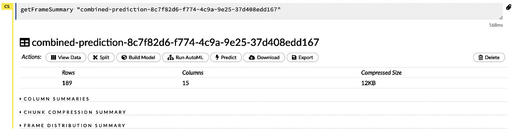
Figure 2.47 – The dataframe used for prediction combined with prediction results
Selecting the View data button in the Actions section of the combined prediction output shows you the complete contents of the dataframe with the predicted values next to it.
The following screenshot shows you the contents of the combined dataframes:
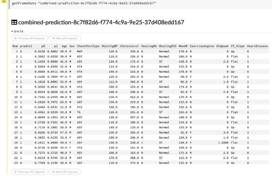
Figure 2.48 – The content of the combined dataframes
Observing the contents of the combined dataframe, you will notice that you can now easily compare the predicted values, as mentioned in the predict column, and compare them with the actual value in the HeartDisease column on the same row.
Congratulations! You have officially made predictions on a model that you trained and combined the results into a single dataframe for a comparative view, which you can share with your stakeholders. So, this sums up our walk-through of how to create an ML pipeline using H2O Flow.
Summary
In this chapter, we understood the various functionality that H2O Flow has to offer. After getting comfortable with the web UI, we started implementing our ML pipeline. We imported and parsed the Heart Failure Prediction dataset. We understood the various operations that can be performed on the dataframe, understood the metadata and statistics of the dataframe, and prepared the dataset to later train, validate, and predict models.
Then, we trained models on the dataframe using AutoML. We understood the various parameters that needed to be input to correctly configure AutoML. We trained models using AutoML and understood the leaderboard. Then, we dived deeper into the details of the models trained and tried our best to understand their characteristics.
Once our model was trained, we performed predictions on it and then explored the prediction output by combining it with the original dataframe so that we could compare the predicted values.
In the next chapter, we will explore the various data manipulation operations further. This will help us to gain an understanding of what steps need to be taken in terms of cleaning and transforming the dataframe and how it could improve the quality of the models trained.