13

Using H2O AutoML with Other Technologies

In the last few chapters, we have been exploring how we can use H2O AutoML in production. We saw how we can use H2O models as POJOs and MOJOs as portable objects that can make predictions. However, in actual production environments, you will often be using multiple technologies to meet various technical requirements. The collaboration of such technologies plays a big role in the seamless functionality of your system.

Thus, it is important to know how we can use H2O models in collaboration with other commonly used technologies in the ML domain. In this chapter, we shall explore and implement H2O with some of these technologies and see how we can build systems that can work together to provide a collaborative benefit.

First, we will investigate how we can host an H2O prediction service as a web service using the Spring Boot application. Then, we will explore how we can perform real-time prediction using H2O with Apache Storm.

In this chapter, we will cover the following topics:

• Using H2O AutoML and Spring Boot
• Using H2O AutoML and Apache Storm

By the end of this chapter, you should have a better understanding of how you can use models trained using H2O AutoML with different technologies to make predictions in different scenarios.

Technical requirements

For this chapter, you will require the following:

• The latest version of your preferred web browser.
• An Integrated Development Environment (IDE) of your choice.
• All the experiments conducted in this chapter have been performed using IntelliJ IDE on an Ubuntu Linux system. You are free to follow along using the same setup or perform the same experiments using IDEs and operating systems that you are comfortable with.

All code examples for this chapter can be found on GitHub at https://github.com/PacktPublishing/Practical-Automated-Machine-Learning-on-H2O/tree/main/Chapter%2013.

Let’s jump right into the first section, where we’ll learn how to host models trained using H2O AutoML on a web application created using Spring Boot.

Using H2O AutoML and Spring Boot

In today’s times, most software services that are created are hosted on the internet, where they can be made accessible to all internet users. All of this is done using web applications hosted on web servers. Even prediction services that use ML can be made available to the public by hosting them on web applications.

The Spring Framework is one of the most commonly used open source web application frameworks to create websites and web applications. It is based on the Java platform and, as such, can be run on any system with a JVM. Spring Boot is an extension of the Spring Framework that provides a preconfigured setup for your web application out of the box. This helps you quickly set up your web application without the need to implement the underlying pipelining needed to configure and host your web service.

So, let’s dive into the implementation by understanding the problem statement.

Understanding the problem statement

Let’s assume you are working for a wine manufacturing company. The officials have a requirement where they want to automate the process of calculating the quality of wine and its color. The service should be available as a web service where the quality assurance executive can provide some information about the wine’s attributes, and the service uses these details and an underlying ML model to predict the quality of the wine as well as its color.

So, technically, we will need two models to make the full prediction. One will be a regression model that predicts the quality of the wine, while the other will be a classification model that predicts the color of the wine.

We can use a combination of the Red Wine Quality and White Wine Quality datasets and run H2O AutoML on it to train the models. You can find the datasets at https://archive.ics.uci.edu/ml/datasets/Wine+Quality. The combined dataset is already present at https://github.com/PacktPublishing/Practical-Automated-Machine-Learning-on-H2O/tree/main/Chapter%2013/h2o_spring_boot/h2o_spring_boot.

The following screenshot shows a sample of the dataset:

Figure 13.1 – Wine quality and color dataset

This dataset consists of the following features:

• fixed acidity: This feature explains the amount of acidity that is non-volatile, meaning it does not evaporate over a certain period.
• volatile acidity: This feature explains the amount of acidity that is volatile, meaning it will evaporate over a certain period.
• citric acid: This feature explains the amount of citric acid present in the wine.
• residual sugar: This feature explains the amount of residual sugar present in the wine.
• chlorides: This feature explains the number of chlorides present in the wine.
• free sulfur dioxide: This feature explains the amount of free sulfur dioxide present in the wine.
• total sulfur dioxide: This feature explains the amount of total sulfur dioxide present in the wine.
• density: This feature explains the density of the wine.
• pH: This feature explains the pH value of the wine, with 0 being the most acidic and 14 being the most basic.
• sulphates: This feature explains the number of sulfates present in the wine.
• alcohol: This feature explains the amount of alcohol present in the wine.
• quality: This is the response column, which notes the quality of the wine. 0 indicates that the wine is very bad, while 10 indicates that the wine is excellent.
• color: This feature represents the color of the wine.

Now that we understand the problem statement and the dataset that we will be working with, let’s design the architecture to show how this web service will work.

Designing the architecture

Before we dive deep into the implementation of the service, let’s look at the overall architecture of how all of the technologies should work together. The following is the architecture diagram of the wine quality and color prediction web service:

Figure 13.2 – Architecture of the wine quality and color prediction web service

Let’s understand the various components of this architecture:

• Client: This is the person – or in this case, the wine quality assurance executive – who will be using the application. The client communicates with the web application by making a POST request to it, passing the attributes of the wine, and getting the quality and color of the wine as a prediction response.
• Spring Boot Application: This is the web application that runs on a web server and is responsible for performing the computation processes. In our scenario, this is the application that will be accepting the POST request from the client, feeding the data to the model, getting the prediction results, and sending the results back to the client as a response.
• Tomcat Web server: The web server is nothing but the software and hardware that handles the HTTP communication over the internet. For our scenario, we shall be using the Apache Tomcat web server. Apache Tomcat is a free and open source HTTP web server written in Java. The web server is responsible for forwarding client requests to the web application.
• Models: These are the trained models in the form of POJOs that will be loaded onto the Spring Boot application. The application will use these POJOs using the h2o-genmodel library to make predictions.
• H2O server: Models will be trained using the H2O server. As we saw in Chapter 1, Understanding H2O AutoML Basics, we can run H2O AutoML on an H2O server. We shall do the same for our scenario by starting an H2O server, training the models using H2O AutoML, and then downloading the trained models as POJOs so that we can load them into the Spring Boot application.
• Dataset: This is the wine quality dataset that we are using to train our models. As stated in the previous section, this dataset is a combination of the Red Wine Quality and White Wine Quality datasets.

Now that we have a good understanding of how we are going to create our wine quality and color prediction web service, let’s move on to its implementation.

Working on the implementation

This service has already been built and is available on GitHub. The code base can be found at https://github.com/PacktPublishing/Practical-Automated-Machine-Learning-on-H2O/tree/main/Chapter%2013/h2o_spring_boot.

Before we dive into the code, make sure your system meets the following minimum requirements:

• Java version 8 and above
• The latest version of Maven, preferably version 3.8.6
• Python version 3.7 and above
• H2O Python library installed using pip3
• Git installed on your system

First, we will clone the GitHub repository, open it in our preferred IDE, and go through the files to understand the whole process. The following steps have been performed on Ubuntu 22.04 LTS and we are using IntelliJ IDEA version 2022.1.4 as the IDE. Feel free to use any IDE of your choice that supports Maven and the Spring Framework for better support.

So, clone the GitHub repository and navigate to Chapter 13/h2o_spring_boot/. Then, you start your IDE and open the project. Once you have opened the project, you should get a directory structure similar to the following:

Figure 13.3 – Directory structure of h2o_wine_predictor

The directory structure consists of the following important files:

• pom.xml: A Project Object Model (POM) is the fundamental unit of the Maven build automation tool. It is an XML file that contains all the information about all the dependencies needed, as well as the configurations needed to correctly build the application.
• script.py: This is the Python script that we will use to train our models on the wine quality dataset. The script starts an H2O server instance, imports the dataset, and then runs AutoML to train the models. We shall look at it in more detail later.
• src/main/java/com.h2o_wine_predictor.demo/api/PredictionController.java: This is the controller file that has the request mapping to direct the POST request to execute the mapped function. The function eventually calls the actual business logic where predictions are made using the ML models and the response is sent back.
• src/main/java/com.h2o_wine_predictor.demo/service/PredictionService.java: This is the actual file where the business logic of making predictions resides. This function imports the POJO models and the h2o-genmodel library and uses them to predict the data received from the controller.
• src/main/java/com.h2o_wine_predictor.demo/Demo: This is the main function of the Spring Boot application. If you want to start the Spring Boot application, you must execute this main function, which starts the Apache Tomcat server that hosts the web application.
• src/main/resources/winequality-combined.csv: This is where the actual CSV dataset is stored. The Python script that trains the H2O models picks the dataset from this path and starts training the models.

You may have noticed that we don’t have the model POJO files anywhere in the directory. So, let’s build those. Refer to the script.py Python file and let’s understand what is being done line by line.

The code for script.py is as follows:

1. The script starts by importing the dependencies:

   import h2o

   import shutil

   from h2o.automl import H2OautoML

2. Once importing is done, the script initializes the H2O server:

   h2o.init()

3. Once the H2O server is up and running, the script imports the dataset from the src/main/resources directory:

   wine_quality_dataframe = h2o.import_file(path = "sec/main/resources/winequality_combined.csv")

4. Since the column color is categorical, the script sets it to factor:

   wine_quality_dataframe["color"] = wine_quality_dataframe["color"].asfactor()

5. Finally, you will need a training and validation DataFrame to train and validate your model during training. Therefore, the script also splits the DataFrame into a 70/30 ratio:

   train, valid = wine_quality_dataframe.split_frame(ratios=[.7])

6. Now that the DataFrames are ready, we can begin the training process for training the first model, which is the classification model to classify the color of the wine. So, the script sets the label and features, as follows:

   label = "color"

   features = ["fixed acidity", "volatile acidity", "citric acid", "residual sugar", "chlorides", "free sulfur dioxide", "total sulfur dioxide", "density", "pH", "sulphates", "alcohol"]

7. Now that the training data is ready, we can create the H2O AutoML object and begin the model training. The following script does this:

   aml_for_color_predictor = H2OAutoML(max_models=10, seed=123, exclude_algos=["StackedEnsemble"], max_runtime_secs=300)

   aml_for_color_predictor.train(x = features, y = label, training_frame=train, validation_frame = valid)

When initializing the H2OautoML object, we set the exclude_algos parameter with the StackedEnsemble value. This is done as stacked ensemble models are not supported by POJOs, as we learned in Chapter 10, Working with Plain Old Java Objects (POJOs).

This starts the AutoML model training process. Some print statements will help you observe the progress and results of the model training process.

8. Once the model training process is done, the script will retrieve the leader model and download it as a POJO with the correct name – that is, WineColorPredictor – and place it in the tmp directory:

   model = aml_for_color_predictor.leader

   model.model_id = "WineColorPredictor"

   print(model)

   model.download_pojo(path="tmp")

9. Next, the script will do the same for the next model – that is, the regression model – to predict the quality of the wine. It slightly tweaks the label and sets it to quality. The rest of the steps are the same:

   label="quality"

   aml_for_quality_predictor = H2OAutoML(max_models=10, seed=123, exclude_algos=["StackedEnsemble"], max_runtime_secs=300)

   aml_for_quality_predictor.train(x = features, y = label, training_frame=train, validation_frame = valid)

10. Once the training is finished, the script will extract the leader model, name it WineQualityPredictor, and download it as a POJO in the tmp directory:

    model = aml_for_color_predictor.leader

    model.model_id = "WineQualityPredictor"

    print(model)

    model.download_pojo(path="tmp")

11. Now that we have both model POJOs downloaded, we need to move them to the src/main/java/com.h2o_wine_predictor.demo/model/ directory. But before we do that, we will also need to add the POJOs to the com.h2o.wine_predictor.demo package so that the PredictionService.java file can import the models. So, the script does this by creating a new file, adding the package inclusion instruction line to the file, appending the rest of the original POJO file, and saving the file in the src/main/java/com.h2o_wine_predictor.demo/model/ directory:

    with open("tmp/WineColorPredictor.java", "r") as raw_model_POJO:

         with open("src/main/java/com.h2o_wine_predictor.demo/model/ WineColorPredictor.java", "w") as model_POJO:

               model_POJO.write(f'package com.h2o_wine_predictor.demo; ' + raw_model_POJO.read())

12. It does the same for the WineQualityPredictor model:

    with open("tmp/WineQualityPredictor.java", "r") as raw_model_POJO:

         with open("src/main/java/com.h2o_wine_predictor.demo/model/ WineQualityPredictor.java", "w") as model_POJO:

               model_POJO.write(f'package com.h2o_wine_predictor.demo; ' + raw_model_POJO.read())

13. Finally, it deletes the tmp directory to clean everything up:

    shutil.rmtree("tmp")

So, let’s run this script and generate our models. You can do so by executing the following command in your Terminal:

python3 script.py

This should generate the respective model POJO files in the src/main/java/com.h2o_wine_predictor.demo/model/ directory.

Now, let’s observe the PredictionService file in the src/main/java/com.h2o_wine_predictor.demo/service directory.

The PredictionService class inside the PredictionService file has the following attributes:

• wineColorPredictorModel: This is an attribute of the EasyPredictModelWrapper type. It is a class from the h2o-genmodel library that is imported by the PredictionService file. We use this attribute to load the WineColorPredictor model that we just generated using script.py. We shall use this attribute to make predictions on the incoming request later.
• wineQualityPredictorModel: Similar to wineColorPredictorModel, this is the wine quality equivalent attribute that uses the same EasyPredictModelWrapper. This attribute will be used to load the WineQualityPredictor model and use it to make predictions on the quality of the wine.

Now that we understand the attributes of this file, let’s check out the methods, which are as follows:

• createJsonResponse(): This function is pretty straightforward in the sense that it takes the binomial classification prediction result from the WineColorPredictor model and the regression prediction result from the WineQualityPredictor model and combines them into a JSON response that the web application sends back to the client.
• predictColor(): This function uses the wineColorPredictorModel attribute of the PredictionService class to make predictions on the data. It outputs the prediction result of the color of the wine as a BinomialModelPrediction object, which is a part of the h2o-genmodel library.
• predictQuality(): This function uses the wineQualityPredictorModel attribute of the PredictionService class to make predictions on the data. It outputs the prediction result of the quality of the wine as a RegressionModelPrediction object, which is part of the h2o-genmodel library.
• fillRowDataFromHttpRequest(): This function is responsible for converting the feature values received from the POST request into a RowData object that will be passed to wineQualityPredictorModel and wineColorPredictorModel to make predictions. RowData is an object from the h2o-genmodel library.
• getPrediction(): This is called by PredictionController, which passes the feature values as a map to make predictions on. This function internally calls all the previously mentioned functions and orchestrates the entire prediction process:

1. It gets the feature values from the POST request as input. It passes these values, which are in the form of Map objects, to fillRowDataFromHttpRequest(), which converts them into the RowData type.
2. Then, it passes this RowData to the predictColor() and predictQuality() functions to get the prediction values.
3. Afterward, it passes these results to the createJsonResponse() function to create an appropriate JSON response with the prediction values and returns the JSON to PredictionController, where the controller returns it to the client.

Now that we have had a chance to go through the important parts of the whole project, let’s go ahead and run the application so that we can have the web service running locally on our machines. Then, we will run a simple cURL command with the wine quality feature values and see if we get the predictions as a response.

To start the application, you can do the following:

• If you are using IntelliJ IDE, then you can directly click on the green play button in the top-right corner of the IDE.
• Alternatively, you can directly run it from your command line by executing the following command inside the project directory where the pom.xml file is:

  mvn spring-boot:run -e

If everything is working fine, then you should get an output similar to the following:

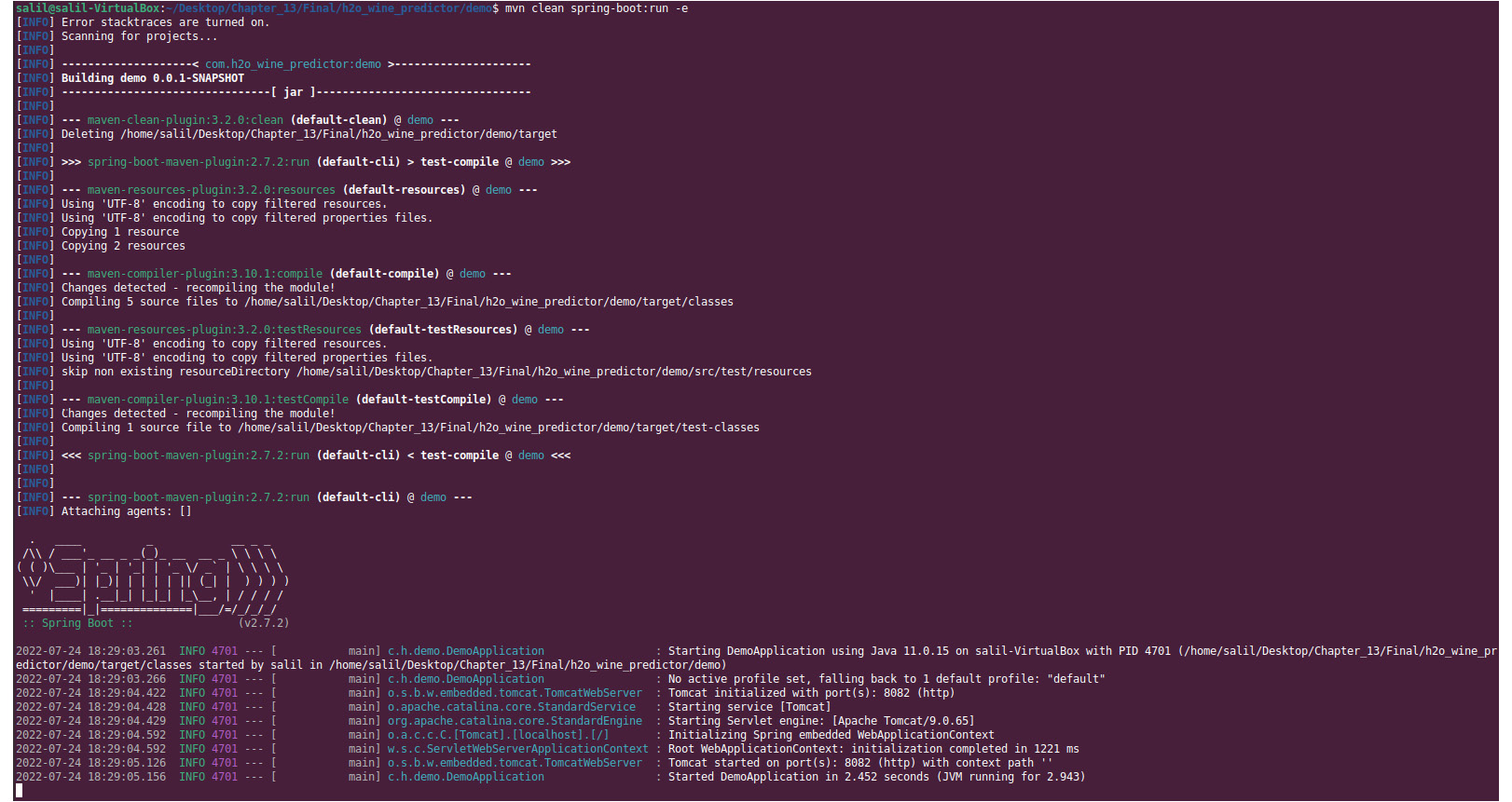
Figure 13.4 – Successful Spring Boot application run output

Now that the Spring Boot application is running, the only thing remaining is to test this out by making a POST request call to the web service running on localhost:8082.

Open another Terminal and execute the following curl command to make a prediction request:

curl -X POST localhost:8082/api/v1/predict -H "Content-Type: application/json" -d '{"fixed acidity":6.8,"volatile acidity":0.18,"citric acid":0.37,"residual sugar":1.6,"chlorides":0.055,"free sulfur dioxide":47,"total sulfur dioxide":154,"density":0.9934,"pH":3.08," ,"sulphates":0.45,"alcohol":9.1}'

The request should go to the web application, where the application will extract the feature values, convert them into the RowData object type, pass RowData to the prediction function, get the prediction results, convert the prediction results into an appropriate JSON, and get the JSON back as a response. This should look as follows:

Figure 13.5 – Prediction result from the Spring Boot web application

From the JSON response, you can see that the predicted color of the wine is white and that its quality is 5.32.

Congratulations! You have just implemented an ML prediction service on a Spring Boot web application. You can further expand this service by adding a frontend that takes the feature values as input and a button that, upon being clicked, creates a POST body of all those values and sends the API request to the backend. Feel free to experiment with this project as there is plenty of scope for how you can use H2O model POJOs on a web service.

In the next section, we’ll learn how to make real-time predictions using H2O AutoML, along with another interesting technology called Apache Storm.

Using H2O AutoML and Apache Storm

Apache Storm is an open source data analysis and computation tool for processing large amounts of stream data in real time. In the real world, you will often have plenty of systems that continuously generate large amounts of data. You may need to make some computations or run some processes on this data to extract useful information as it is generated in real time.

What is Apache Storm?

Let’s take the example of a log system in a very heavily used web service. Assuming that this web service receives millions of requests per second, it is going to generate tons of logs. And you already have a system in place that stores these logs in your database. Now, this log data will eventually pile up and you will have petabytes of log data stored in your database. Querying all this historical data to process it in one go is going to be very slow and time-consuming.

What you can do is process the data as it is generated. This is where Apache Storm comes into play. You can configure your Apache Storm application to perform the needed processing and direct your log data to flow through it and then store it in your database. This will streamline the processing, making it real-time.

Apache Storm can be used for multiple use cases, such as real-time analytics, Extract-Transform-Load (ETL) data in data pipelines, and even ML. What makes Apache Storm the go-to solution for real-time processing is because of how fast it is. A benchmarking test performed by the Apache Foundation found Apache Storm to process around a million tuples per second per node. Apache Storm is also very scalable and fault-tolerant, which guarantees that it will process all the incoming real-time data.

So, let’s dive deep into the architecture of Apache Storm to understand how it works.

Understanding the architecture of Apache Storm

Apache Storm uses cluster computing, similar to how Hadoop and even H2O work. Consider the following architectural diagram of Apache Storm:

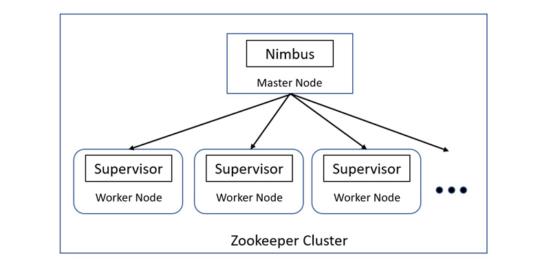
Figure 13.6 – Architecture of Apache Storm

Apache Storm distinguishes the nodes in its cluster into two categories – a master node and a worker node. The features of these nodes are as follows:

• Master Node: The master node runs a special daemon called Nimbus. The Nimbus daemon is responsible for distributing the data among all the worker nodes in the cluster. It also monitors failures and will resend the data to other nodes once a failure is detected, ensuring that no data is left out of processing.
• Worker Node: The worker nodes run a daemon called the Supervisor. The Supervisor daemon is the service that is constantly listening for work and starts or stops the underlying processes as necessary for the computation.

The communication between the master node and the worker nodes using their respective daemons is done using the Zookeeper cluster. In short, the Zookeeper cluster is a centralized service that maintains configuration and synchronization services for stateless groups. In this scenario, the master node and the worker nodes are stateless and fast-failing services. All the state details are stored in the Zookeeper cluster. This is beneficial as keeping the nodes stateless helps with fault tolerance as the nodes can be brought back to life and they will start working as if nothing had happened.

Tip

If you are interested in understanding the various concepts and technicalities of Zookeeper, then feel free to explore it in detail at https://zookeeper.apache.org/.

Before we move on to the implementation part of Apache Storm, we need to be aware of certain concepts that are important to understand how Apache Storm works. The different concepts are as follows:

• Tuples: Apache Storm uses a data model called Tuple as its primary unit of data that is to be processed. It is a named list of values and can be an object of any type. Apache Storm supports all primitive data types out of the box. But it can also support custom objects, which can be deserialized into primitive types.
• Streams: Streams are unbounded sequences of tuples. A stream represents the path from where your data flows from one transformation to the next. The basic primitives that Apache Storm provides for doing these transformations are spouts and bolts:
  • Spouts: A spout is a source for a stream. It is at the start of the stream from where it reads the data from the outside world. It takes this data from the outside world and sends it to a bolt.
  • Bolt: A bolt is a process that consumes data from single or multiple streams, transforms or processes it, and then outputs the result. You can link multiple bolts one after the other while feeding the output of one bolt as input to the next to perform complex processing. Bolts can run functions, filter data, perform aggregation, and even store data in databases. You can perform any kind of functionality you want on a bolt.
• Topologies: The entire orchestration of how data will be processed in real time using streams, spouts, and bolts in the form of a Directed Acyclic Graph (DAG) is called a topology. You need to submit this topology to the Nimbus daemon using the main function of Apache Storm. The topology graph contains nodes and edges, just like a regular graph structure. Each node contains processing logic and each edge shows how data is to be transferred between two nodes. Both the Nimbus and the topology are Apache Thrift structures, which are special type systems that allow programmers to use native types in any programming language.

Tip

You can learn more about Apache Thrift by going to https://thrift.apache.org/docs/types.

Now that you have a better understanding of what Apache Storm is and the various concepts involved in its implementation, we can move on to the implementation part of this section, starting with installing Apache Storm.

Tip

Apache Storm is a very powerful and sophisticated system. It has plenty of applicability outside of just machine learning and also has plenty of features and support. If you want to learn more about Apache Storm, go to https://storm.apache.org/.

Installing Apache Storm

Let’s start by noting down the basic requirements for installing Apache Storm. They are as follows:

• Java version greater than Java 8
• The latest version of Maven, preferably version 3.8.6

So, make sure these basic requirements are already installed on your system. Now, let’s start by downloading the Apache Storm repo. You can find the repo at https://github.com/apache/storm.

So, execute the following command to clone the repository to your system:

git clone https://github.com/apache/storm.git

Once the download is finished, you can open the storm folder to get a glimpse of its contents. You will notice that there are tons of files, so it can be overwhelming when you’re trying to figure out where to start. Don’t worry – we’ll work on very simple examples that should be enough to give you a basic idea of how Apache Storm works. Then, you can branch out from there to get a better understanding of what Apache Storm has to offer.

Now, open your Terminal and navigate to the cloned repo. You will need to locally build Apache Storm itself before you can go about implementing any of the Apache Storm features. You need to do this as locally building Apache Storm generates important JAR files that get installed in your $HOME/.m2/repository folder. This is the folder where Maven will pick up the JAR dependencies when you build your Apache Storm application.

So, locally build Apache Storm by executing the following command at the root of the repository:

mvn clean install -DskipTests=true

The build might take some time, considering that Maven will be building several JAR files that are important dependencies to your application. So, while that is happening, let’s understand the problem statement that we will be working on.

Understanding the problem statement

Let’s assume you are working for a medical company. The medical officials have a requirement, where they want to create a system that predicts whether the person is likely to suffer from any complications after surviving a heart failure or whether they are safe to be discharged. The catch is that this prediction service will be used by all the hospitals in the country, and they need immediate prediction results so that the doctors can decide whether to keep the patient admitted for a few days to monitor their health or decide to discharge them.

So, the machine learning problem is that there will be streams of data that our system will need to make immediate predictions. We can set up a Apache Storm application that streams all the data into the prediction service and deploys model POJOs trained using H2O AutoML to make the predictions.

We can train the models on the Heart Failure Clinical dataset, which can be found at https://archive.ics.uci.edu/ml/datasets/Heart+failure+clinical+records.

The following screenshot shows some sample content from the dataset:

Figure 13.7 – Heart Failure Clinical dataset

This dataset consists of the following features:

• age: This feature indicates the age of the patient in years
• anemia: This feature indicates the decrease of red blood cells or hemoglobin, where 1 indicates yes and 0 indicates no
• high blood pressure: This feature indicates if the patient has hypertension, where 1 indicates yes and 0 indicates no
• creatinine phosphokinase: This feature indicates the level of the CPK enzyme in the blood in micrograms per liter (mcg/L)
• diabetes: This feature indicates if the patient has diabetes, where 1 indicates yes and 0 indicates no
• ejection fraction: This feature indicates the percentage of blood leaving the heart at each contraction
• platelets: This feature indicates the platelets in the blood in kilo platelets per milliliter (ml)
• sex: This feature indicates if the patient is a man or woman, where 1 indicates the patient is a woman and 0 indicates the patient is a man
• serum creatinine: This feature indicates the level of serum creatinine in the blood in milligrams per deciliter (mg/dL)
• serum sodium: This feature indicates the level of serum sodium in the blood milliequivalent per liter (mEq/L)
• smoking: This feature indicates if the patient smokes or not, where 1 indicates yes and 0 indicates no
• time: This feature indicates the number of follow-ups in days
• complications: This feature indicates if the patient faced any complications during the follow-up period, where 1 indicates yes and 0 indicates no

Now that we understand the problem statement and the dataset that we will be working with, let’s design the architecture of how we can use Apache Storm and H2O AutoML to solve this problem.

Designing the architecture

Let’s look at the overall architecture of how all the technologies should work together. Refer to the following architecture diagram of the heart failure complication prediction service:

Figure 13.8 – Architecture diagram of using H2O AutoML with Apache Storm

Let’s understand the various components of the architecture:

• script.py: From an architectural point of view, the solution is pretty simple. First, we train the models using H2O AutoML, which can be easily done by using this script, which imports the dataset, sets the label and features, and runs AutoML. The leader model can then be extracted as a POJO, which we can later use in Apache Storm to make predictions.
• Data Spout: We will have a spout in Apache Storm that constantly reads data and passes it to the Prediction Bolt in real time.
• Prediction Bolt: This bolt contains the prediction service that imports the trained model POJO and uses it to make predictions.
• Classification Bolt: The results from the Prediction Bolt are passed to this bolt. This bolt classifies the results as potential complications and no complications based on the binary classification result from the Prediction Bolt.

Now that we have designed a simple and good solution, let’s move on to its implementation.

Working on the implementation

This service is already available on GitHub. The code base can be found at https://github.com/PacktPublishing/Practical-Automated-Machine-Learning-on-H2O/tree/main/Chapter%2013/h2o_apache_storm/h2o_storm.

So, download the repo and navigate to /Chapter 13/h2o_apache_storm/h2o_storm/.

You will see that we have two folders. One is the storm-starter directory, while the other is the storm-streaming directory. Let’s focus on the storm-streaming directory first. Start your IDE and open the storm-streaming project. Once you open the project, you should see a directory structure similar to the following:

Figure 13.9 – storm_streaming directory structure

This directory structure consists of the following important files:

• scripty.py: This is the Python script that we will use to train our models on the heart failure complication dataset. The script starts an H2O server instance, imports the dataset, and then runs AutoML to train the models. We shall look at this in more detail later.
• H2ODataSpout.java: This is the Java file that contains the Apache Storm spout and its functionality. It reads the data from the live_data.csv file and forwards individual observations one at a time to the bolts, simulating the real-time flow of data.
• H2OStormStarter.java: This is a Java file that contains the Apache Storm topology with the two bolts – the Prediction Bolt and Classification Bolt classes. We shall start our Apache Storm service using this file.
• training_data.csv: This is the dataset that contains a part of the heart failure complication data that we will be using to train our models.
• live_data.csv: This is the dataset that contains the heart failure complication data that we will be using to simulate the real-time inflow of data into our Apache Storm application.

Unlike the previous experiments, where we made changes in a separate application repository, for this experiment, we shall make changes in Apache Storm’s repository.

The following steps have been performed on Ubuntu 22.04 LTS; IntelliJ IDEA version 2022.1.4 has been used as the IDE. Feel free to use any IDE of your choice that supports the Maven framework for better support.

Let’s start by understanding the model training script, script.py. The code for script.py is as follows:

1. First, the script imports the dependencies:

   import h2o

   from h2o.automl import H2OautoML

2. Once importing is done, the H2O server is initialized:

   h2o.init()

3. Once the H2O server is up and running, the script imports the training_data.csv file:

   wine_quality_dataframe = h2o.import_file(path = "training_data.csv")

4. Now that the DataFrame has been imported, we can begin the training process for training the models using AutoML. So, the script sets the label and features, as follows:

   label = "complications"

   features = ["age", "anemia", "creatinine_phosphokinase", "diabetes", "ejection_fraction", "high_blood_pressure", "platelets", "serum_creatinine ", "serum_sodium", "sex", "smoking", "time"]

5. Now, we can create the H2O AutoML object and begin the model training:

   aml_for_complications = H2OAutoML(max_models=10, seed=123, exclude_algos=["StackedEnsemble"], max_runtime_secs=300)

   aml_for_complications.train(x = features, y = label, training_frame = wine_quality_dataframe )

Since POJOs are not supported for stacked ensemble models, we set the exclude_algos parameter with the StackedEnsemble value.

This starts the AutoML model training process. Some print statements are in here that will help you observe the progress and results of the model training process.

6. Once the model training process is done, the script retrieves the leader model and downloads it as a POJO with the correct name – that is, HeartFailureComplications – and places it in the tmp directory:

   model = aml_for_color_predictor.leader

   model.model_id = "HeartFailureComplications"

   print(model)

   model.download_pojo(path="tmp")

So, let’s run this script and generate our model. Executing the following command in your Terminal:

python3 script.py

This should generate the respective model POJO files in the tmp directory.

Now, let’s investigate the next file in the repository: H2ODataSpout.java. The H2ODataSpout class in the Java file has a few attributes and functions that are important for building the Apache Storm applications. We won’t focus on them much, but let’s have a look at the functions that do play a bigger role in the business logic of the applications. They are as follows:

• nextTuple(): This function contains the logic of reading the data from the live_data.csv file and emits the data row by row to the Prediction Bolt. Let’s have a quick look at the code:
  1. First, you have the sleep timer. Apache Storm, as we know, is a super-fast real-time data processing system. Observing our live data flowing through the system will be difficult for us, so the sleep function ensures that there is a delay of 1,000 milliseconds so that we can easily observe the flow of data and see the results:

  Util.sleep(1000)

2. The function then instantiates the live_data.csv file into the program:

File file = new File("live_data.csv")

3. The code then declares the observation variable. This is nothing but the individual row data that will be read and stored in this variable by the spout:

String[] observation = null;

4. Then, we have the logic where the spout program reads the row in the data. Which row to read is decided by the _cnt atomic integer, which gets incremented as the spout reads and emits the row to the Prediction Bolt in an infinite loop. This infinite loop simulates the continuous flow of data, despite live_data.csv containing only limited data:

try {

      String line="";

      BufferedReader br = new BufferedReader(new FileReader(file));

      while (i++<=_cnt.get()) line = br.readLine(); // stream thru to next line

      observation = line.split(",");

    } catch (Exception e) {

      e.printStackTrace();

      _cnt.set(0);

    }

5. Then, we have the atomic number increment so that the next iteration picks up the next row in the data:

_cnt.getAndIncrement();

if (_cnt.get() == 1000) _cnt.set(0);

6. Finally, we have the _collector.emit() function, which emits the row data so that it’s stored in _collector, which, in turn, is consumed by the Prediction Bolt:

_collector.emit(new Values(observation));

• declareOutputFields(): In this method, we declare the headers of our data. We can extract and use the headers from our trained AutoML model POJO using its NAMES attribute:

  LinkedList<String> fields_list = new LinkedList<String>(Arrays.asList(ComplicationPredictorModel.NAMES));

  fields_list.add(0,"complication");

  String[] fields = fields_list.toArray(new String[fields_list.size()]);

  declarer.declare(new Fields(fields));

• Other miscellaneous functions: The remaining open(), close(), ack(), fail(), and getComponentConfiguration() functions are supportive functions for error handling and preprocessing or postprocessing activities that you might want to do in the spout. To keep this experiment simple, we won’t dwell on them too much.

Moving on, let’s investigate the H2OStormStarter.java file. This file contains both bolts that are needed for performing the predictions and classification, as well as the h2o_storm() function, which builds the Apache Storm topology and passes it onto the Apache Storm cluster. Let’s dive deep into the individual attributes:

• class PredictionBolt: This is the Bolt class and is responsible for obtaining the class probabilities of the heart failure complication dataset. It imports the H2O model POJO and uses it to calculate the class probabilities of the incoming row data. It has three functions – prepare(), execute() and declareOutputFields(). We shall only focus on the execute function since it contains the execution logic of the bolt; the rest are supportive functions. The execute function contains the following code:
  1. The very first thing this function does is import the H2O model POJO:

  HeartFailureComplications h2oModel = new HeartFailureComplications();

2. Then, it extracts the input tuple values from its parameter variables and stores them in the raw_data variable:

ArrayList<String> stringData = new ArrayList<String>();

for (Object tuple_value : tuple.getValues()) stringData.add((String) tuple_value);

String[] rawData = stringData.toArray(new String[stringData.size()]);

3. Next, the code categorically maps all the categorical data in the row:

double data[] = new double[rawData.length-1];

String[] columnName = tuple.getFields().toList().toArray(new String[tuple.size()]);

for (int I = 1; i < rawData.length; ++i) {

   data[i-1] = h2oModel.getDomainValues(columnName[i]) == null

             ? Double.valueOf(rawData[i])

            : h2oModel.mapEnum(h2oModel.getColIdx(columnName[i]), rawData[i]);

}

4. Then, the code gets the prediction and emits the results:

double[] predictions = new double [h2oModel.nclasses()+1];

h2oModel.score0(data, predictions);

_collector.emit(tuple, new Values(rawData[0], predictions[1]));

5. Finally, the code acknowledges the tuple so that the spout is informed about its consumption and won’t resend the tuple for retry:

_collector.ack(tuple);

• Classifier Bolt: This bolt receives the input from the Prediction Bolt. The functionality of this bolt is very simple: it takes the class probabilities from the input and compares them against the threshold value to determine what the predicted outcome will be. Similar to the Prediction Bolt, this Bolt class also has some supportive functions, along with the main execute() function. Let’s dive deep into this to understand what is going on in the function:
  • The function simply computes if there is a possibility of Possible Complication or No Complications based on the _threshold value and emits the result back:

    _collector.emit(tuple, new Values(expected, complicationProb <= _threshold ? "No Complication" : "Possible Complication"));

    _collector.ack(tuple);

• h2o_storm(): This is the main function of the application and builds the topology using H2ODataSpout and the two bolts – Prediction Bolt and Classifier Bolt. Let’s have a deeper look into its functionality.
  1. First, the function instantiates TopologyBuilder():

  TopologyBuilder builder = new TopologyBuilder();

2. Using this object, it builds the topology by setting the spout and the bolts, as follows:

builder.setSpout("inputDataRow", new H2ODataSpout(), 10);

builder.setBolt("scoreProbabilities", new PredictionBolt(), 3).shuffleGrouping("inputDataRow");

builder.setBolt("classifyResults", new ClassifierBolt(), 3).shuffleGrouping("scoreProbabilities");

3. Apache Storm also needs some configuration data to set up its cluster. Since we are creating a simple example, we can just use the default configurations, as follows:

Config conf = new Config();

4. Finally, it creates a cluster and submits the topology it created, along with the configuration:

LocalCluster cluster = new LocalCluster();

cluster.submitTopology("HeartComplicationPredictor", conf, builder.createTopology());

5. After that, there are some functions to wrap the whole experiment together. The Util.sleep() function is used to pause for an hour so that Apache Storm can loop over the functionality indefinitely while simulating a continuous flow of real-time data. The cluster.killTopology() function kills the HeartComplicationPredictor topology, which stops the simulation in the cluster. Finally, the cluster.shutdown() function brings down the Apache Storm cluster, freeing up the resources:

Utils.sleep(1000 * 60 * 60);

cluster.killTopology("HeartComplicationPredictor");

cluster.shutdown();

Now that we have a better understanding of the contents of the files and how we are going to be running our service, let’s proceed and look at the contents of the storm-starter project. The directory structure will be as follows:

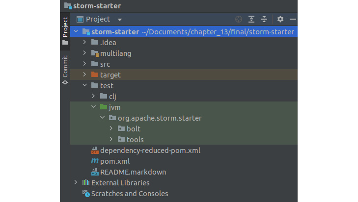
Figure 13.10 – storm-starter directory structure

The src directory contains several different types of Apache Storm topology samples that you can choose to experiment with. I highly recommend that you do so as that will help you get a better understanding of how versatile Apache Storm is when it comes to configuring your streaming service for different needs.

However, we shall perform this experiment in the test directory to keep our files isolated from the ones in the src directory. So, let’s see how we can run this experiment.

Follow these steps to build and run the experiment:

1. In the storm-streaming directory, run the script.py file to generate the H2O model POJO. The script should run H2O AutoML and generate a leaderboard. The leader model will be extracted, renamed HeartFailureComplications, and downloaded as a POJO. Run the following command in your Terminal:

   python3 script.py

2. The HeartFailureComplications POJO will be imported by the other files in the storm-starter project, so to ensure that it can be correctly imported by files in the same package, we need to add this POJO to that same package. So, modify the POJO file to add the storm.starter package as the first line.
3. Now, move the HeartFailureComplications POJO file, the H2ODataSpout.java file, and the H2OStormStarted.java file inside the storm-starter repository inside its storm-starter/test/jvm/org.apache.storm.starter directory.
4. Next, we need to import the h2o-model.jar file into the storm-starter project. We can do so by adding the following dependency to the pom.xml file of the experiment, as follows:

   <dependency>

       <groupId>ai.h2o</groupId>

       <artifactId>h2o-genmodel</artifactId>

       <version>3.36.1.3</version>

   </dependency>

Your directory should now look as follows:

Figure 13.11 – storm-starter directory structure after file transfers

5. Finally, we will run this project by right-clicking on the H2OStormStarter.java file and running it. You should get a stream of constant output that demonstrates your spout and bolt in action. This can be seen in the following screenshot:

Figure 13.12 – Heart complication prediction output in Apache Storm

If you observe the results closely, you should see that there are executors in the logs; all the Apache Storm spouts and bolts are internal executor processes that run on the cluster. You will also see the prediction probabilities besides each tuple. This should look as follows:

Figure 13.13 – Heart complication prediction result

Congratulations – we have just covered another design pattern that shows us how we can use models trained using H2O AutoML to make real-time predictions on streaming data using Apache Storm. This concludes the last experiment of this chapter.

Summary

In this chapter, we focused on how we can implement models that have been trained using H2O AutoML in different scenarios using different technologies to make predictions on different kinds of data.

We started by implementing an AutoML leader model in a scenario where we tried to make predictions on data over a web service. We created a simple web service that was hosted on localhost using Spring Boot and the Apache Tomcat web server. We trained the model on data using AutoML, extracted the leader model as a POJO, and loaded that POJO as a class in the web application. By doing this, the application was able to use the model to make predictions on the data that it received as a POST request, responding with the prediction results.

Then, we looked into another design pattern where we aimed to make predictions on real-time data. We had to implement a system that can simulate the real-time flow of data. We did this with Apache Storm. First, we dived deep into understanding what Apache Storm is, its architecture, and how it works by using spouts and bolts. Using this knowledge, we built a real-time data streaming application. We deployed our AutoML trained model in a Prediction Bolt where the Apache Storm application was able to use the model to make predictions on the real-time streaming data.

This concludes the final chapter of this book. There are still innumerable features, concepts, and design patterns that we can work with while using H2O AutoML. The more you experiment with this technology, the better you will get at implementing it. Thus, it is highly recommended that you keep experimenting with this technology and discover new ways of solving ML problems while automating your ML workflows.