
Chapter 6
Advanced Topics in Predictive Modeling
Predictive analytics is still as much of an art as it is science. For a given business problem and a set of real world data, developing predictive analytics and machine learning models that are capable of producing highly accurate and unbiased predictions, that are interpretable and explainable by humans, while computationally efficient and easily deployable is a challenging task for any data scientist. Although we have seen significant improvements in the standardization and automation of methodologies (as depicted in the CRISP methodology; see Chapter 3) and creation of best/better practices for model building in recent years, the true optimization of the complete data science / business analytics process still remains as a eutopia. Many, including the author of this book believes that at best we are halfway through in achieving this endeavour. In this chapter, we cover some of the relatively novel concepts and approaches proposed to pave the road towards achieving the eutopia. Specifically, this chapter covers in due details the ensemble modeling, bias-variance tradeoff, how to handle the class imbalance problem and the human interpretability of machine learning models.
Model Ensembles
Ensembles (or more appropriately called as model ensembles or ensemble modeling) is a relatively new practice in data science and predictive modelling where outcomes produced by two or more analytics models are combined into a compound output. Ensembles are primarily used for prediction modeling where the scores of two or more model are combined to produce a better prediction. The prediction can be either classification or regression/estimation type (i.e., former predicting a class label while latter estimating a numerical output variable). Although use of ensembles has been dominated by prediction type modeling, it can also be used for other analytics tasks such as clustering and association rule mining. That is, model ensembles can be used for supervised as well as unsupervised machine learning tasks. Traditionally these machine learning procedures focused on identifying and building the best possible model (often the most accurate predictor on the holdout data) from a large number of alternative model types. To do so, analysts and scientist used an elaborate experimental process that mainly relied on trial-and-error to improve each single model’s performance (defined by some predetermined metrics, e.g., prediction accuracy) to its best possible level so that the best of the models can be used/deployed for the task at hand. The ensemble approach turns this thinking around. Rather than building models and selecting the single best model to use/deploy, it proposes to build many models and use them all for the task they are intended to perform (e.g., prediction).
Motivation—Why Do We Need Model Ensembles?
Usually researcher and practitioners build ensembles for two main reasons: better accuracy and more stable/robust/ consistent/reliable outcomes. Numerous research studies and publications over the past two decades have shown that ensembles almost always improve predictive accuracy for the given problem and rarely predict worse than the single models (Abbott, 2014). Ensembles began to appear in the data mining/analytics literature in 1990s, motivated by the limited success obtained by the earlier works on combining forecasts that dated a couple of more decades. By the early-to-mid 2000s, ensembles became popular and almost essential to winning data mining and predictive modeling competitions. One of the most popular examples of ensembles winning competitions is perhaps the famous Netflix prize, which was an open competition that solicited researcher and practitioners to predict user ratings of films based on historical ratings. The prize was 1 Million USD for a team that could reduce the root means squared error (RMSE) of the then-existing Netflix internal prediction algorithm by the largest margin but no less than 10 percentage point. The winner, runner-up, and nearly all the teams at the top of the leaderboard used model ensembles in their submissions. As a result, the winning submission was the result of an ensemble containing hundreds of predictive models.
When it comes to justifying the use of ensembles Vorhies (2016) puts it the best—if you want to win a predictive analytics competition (at Kaggle or at anywhere else) or at least get a respectable place on the leader board, you are to embrace and intelligently use model ensembles. Kaggle has become the premier platform for data scientist to showcase their talents. According to Vorhies, the Kaggle competitions are like formula racing for data science. Winners edge out competitors at the fourth decimal place and like Formula-1 race cars, not many of us would mistake them for daily drivers. The amount of time devoted and the extreme techniques used would not always be appropriate for an ordinary data science production project, but like paddle shifters and exotic suspensions, some of those improvements and advanced features find their way into day-to-day life and practice of analytics professionals. In addition to Kaggle competitions, reputable associations such as the Association for Computing Machinery (ACM)’s Special Interest Group (SIG) on Knowledge Discovery and Data Mining (SIGKDD) and Pacific-Asia Conference in Knowledge Discovery and Data Mining (PAKDD) regularly organizes competition (often called “cups”) for the community of data scientists to demonstrate their competences, sometimes for monetary rewards but most often for simple bragging rights. Some of the popular analytics companies like SAS Institute and Teradata Corporation organize similar competitions for (and extends variety of relatively modest awards to) both graduate and undergraduate students in universities all over the world, usually in concert with their regular analytics conferences.
It is not just the accuracy that makes model ensembles popular and unavoidably necessary. Yes, it has been shown time and time again that ensembles can improve model accuracy, but they can also improve model robustness, stability, and hence, reliability. This advantage of model ensembles is equally (or perhaps more) important and invaluable than accuracy in situations where reliable prediction is of the essence. In ensemble models, through combining (some form of averaging) multiple models into a single prediction outcome, no single model dominates the final predicted value of the models, which in turn, reduces the likelihood of making a way-off-target “wacky” prediction. Figure 6.1 shows a graphical illustration of model ensembles for classification type prediction problems. Although some varieties exist, most ensemble modeling methods follow this generalized process. From left to right, Figure 6.1 illustrates the general tasks of data acquisition and data preparation, followed by cross-validation and model building-and-testing, and finally assembling/combining the individual model outcomes and assessing the resultant predictions.

Figure 6.1 A graphical depiction of model ensembles for prediction modeling
Another way to look at ensembles is from the perspective of “collective wisdom” or “crowdsourcing.” In the popular book The Wisdom of Crowds (Surowiecki, 2005), the author proposes that better decisions can be made if (rather than relying on a single expert) many (even uninformed) opinions can be aggregated into a decision that is superior to the best expert’s opinion, often called crowdsourcing. In his book Surowiecki describes four characteristics necessary for the group opinion to work well and not degenerate into the opposite effect of poor decisions as evidenced by the “madness of crowds”: diversity of opinion, independence, decentralization, and aggregation. The first three characteristics relate to how the individual decisions are made—they must have information different than others in the group and not be affected by the others in the group. The last characteristic merely states that the decisions must be combined. These four principles/characteristics seem to lay the foundation for building better model ensembles as well. Each predictive model has a voice in the final decision. The diversity of opinion can be measured by the correlation of the predictive values themselves—if all of the predictions are highly correlated with one another, or in other words, if the models nearly all agree, there is no foreseeable advantage in combining them. The decentralization characteristic can be achieved by resampling data or through case weights—each model uses either different records from a common data set or at least uses the records with weights that are different from the other models (Abbott, 2014).
One of the prevalent concepts in statistics and predicate modeling that is highly relevant to model ensembles is the bias-variance tradeoff. Therefore, before delving into the different types of model ensembles, it is necessary to review and understand the bias-variance tradeoff principle (as it applied to the field of statistics or machine-learning). In predictive analytics, bias refers to the error and variance refers to the consistency (or lack thereof) in predictive accuracy of models applied to other data sets. The best models expected to have low bias (low error, high accuracy) and low variance (consistency of accuracy from data set to data set). Unfortunately, there is always a tradeoff between these two metrics in building predictive models—improving one results in worsening the other. You can achieve low bias on training data, but the model may suffer from high variance on hold-out/validation data because the models may have been over-trained/overfit. For instance, the kNN algorithm with k = 1 is an example of a low bias model (perfect on training data set), but susceptible to high variance on test/validation data set. Use of cross validation along with proper model ensembles seems to be the current best practice in handling such tradeoff between bias and variance in predictive modeling.
Types of Model Ensembles
Ensembles, or teams of predictive models working together, have been the fundamental strategy for developing accurate and robust analytics models. Although they have been around for quite a while, their popularity and effectiveness has surfaced in a significant way only within the last decade, as they continually improved in parallel to the rapidly improving software and hardware capabilities. When we say model ensembles, many of us immediately think of decision-tree ensembles like random forest and boosted trees, however, generally speaking the model ensembles can be classified into four groups in two dimensions, as shown in Figure 6.2. The first dimension is the method type (the x-axis in Figure 6.2), where the ensembles can be grouped into bagging or boosting types. The second dimension is the model type (the y-axis in Figure 6.2), where the ensembles can be grouped into homogeneous or heterogeneous types (Abbott, 2014).
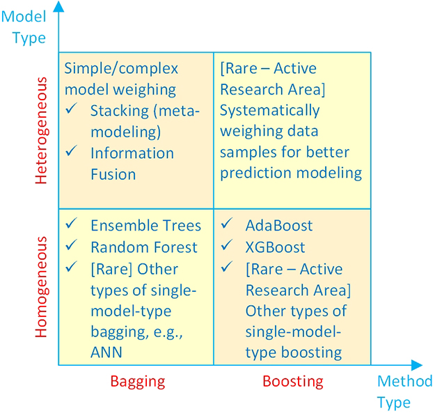
Figure 6.2 A simple taxonomy for model ensembles
As the name implies, homogeneous type ensembles combine the outcomes of two or more of the same type of models such as decision trees. In fact, a vast majority of homogeneous model ensembles are developed using a combination of decision tree structures. The two most common categories of homogeneous type ensembles that use decision trees are bagging and boosting (more information on these are given later in this chapter). Heterogeneous model ensembles, again as the name implies, combines the outcomes of two or more different types of models such as decision trees, artificial neural networks, logistic regression, support vector machines, and others. As mentioned in the context of “the wisdom of crows,” one of the key success factors in ensemble modeling is to use models that are of fundamentally different from one another, ones that look at the data from a different perspective. Because of the way it combines the outcomes of different model types, heterogeneous model ensembles are also called information fusion models (Delen & Sharda, 2010) or stacking (more information on these are given later in this chapter).
Bagging
Bagging is the simplest and most common ensemble method. Leo Brieman, a very well-respected scholar in the world of statistics and analytics, is known to have first published a description of the bagging (i.e., Bootstrap Aggregating) algorithm at Berkeley in 1996 (Breiman, 1996). The idea behind begging is quite simple yet powerful: build multiple decision trees from resampled data and combine the predicted values through averaging or voting. The resampling method Breiman used was bootstrap sampling (sampling with replacement), which creates replicates of some records in the training data. With this selection method, on average, about 37 percent of the records will not be included at all in the training data set (Abbott, 2014).
Although bagging was first developed for decision trees, the idea can be applied to any predictive modeling algorithm that produces outcomes with sufficient variation in the predicted values. Although rare in practice, the other predictive modeling algorithm that are potential candidates for bagging type model ensembles include neural networks, Naiïve Bayes, k-nearest neighbor (for low values of k), and to a lesser degree, even logistic regression. k-nearest neighbor is not a good candidate for bagging if the value of k is already large; the algorithm already votes or aver- ages predictions and with larger values of k, predictions are already very stable with low variance.
Bagging can be used for both classification and regression/estimation type prediction problems. In classification type prediction problems, all of the participant models’ outcomes (class assignments) are combined using an either simple or complex/weighted majority voting mechanism. The class label that gets the most/highest votes becomes the aggregated/ensemble prediction for that sample/record. In regression/estimation type prediction problem where the output/target variable is a number, all of the participant models’ outcomes (numerical estimations) are combined using an either simple or complex/weighted averaging mechanism. Figure 6.3 illustrates the graphical depiction of a decision tree type bagging algorithm.

Figure 6.3 Bagging type decision tree ensembles
One of the key questions in begging is “how many bootstrap samples, also called replicates, should be created?” Brieman stated, “my sense of it is that fewer are required when y [dependent variable] is numerical and more are required with an increasing number of classes [for classification type prediction problems].” He typically used 10–25 bootstrap replicates, with significant improvements occurring with as few as 10 replicates. Overfitting the models is an important requirement to building good bagged ensembles. By overfitting each model, the bias is low, but the decision tree will generally have worse accuracy on held-out data. But bagging is a variance reduction technique; the averaging of predictions smoothes the predictions to behave in a more stable way on new data.
As mentioned before, the diversity of model predictions is a key factor in creating effective ensembles. One way to measure the diversity of predictions is to examine the correlation of predicted values. If the correlations between model predictions are always very high, greater than 0.95, there is little additional predictive information each model brings to the ensemble and therefore little improvement in accuracy is achievable. Generally, it is best to have correlations less than 0.9 at most. The correlations should be computed from the model propensities or predicted probabilities rather than the {0,1} classification value itself. Bootstrap sampling in bagging is the key to introducing diversity in the models. One can think of the bootstrap sampling methodology as creating case weights for each record—some records are included multiple times in the training data (their weights are 1, 2, 3, or more) and others are not included at all (their weights are equal to 0) (Abbott, 2014).
Boosting
Boosting is another, perhaps second most common after bagging, ensemble method. Yoav Freund and Robert E. Schapire are known to have first introduced the boosting algorithm in separate publications in early 1990s, and then in a 1996 in a joint publication (Yoav and Schapire, 1996), they introduced the well-known boosting algorithm, called AdaBoost. As was in bagging, the idea behind bagging is also quite straightforward. First, build a rather simple classification model; the model only needs to be slightly better than random chance, so for a binary classification problem, only slightly better than a 50 percent correct classification. In this first pass, each record is used in the algorithm with equal case weights, as one would do normally in building a predictive model. The errors in the predicted values for each case are noted. The correctly classified records/cases/samples will have their case weights stay the same, or perhaps reduced, and the records that are incorrectly classified will have their case weights increased, and then a second simple model is built on these weighted cases (i.e., the transformed/weighted training dataset). In other words, for the second model, records that were incorrectly classified are “boosted” through case weights to be considered more strongly or seriously in the construction of the new prediction model. In each iteration, the records that are incorrectly predicted (the ones that are difficult to classify), keep getting case weights increased, communicating to the algorithm to pay more attention to these records until, hopefully, they are finally classified correctly.
This process of boosting is often repeated tens or even hundreds of times. After the tens or hundreds of iterations, the final predictions are made based on a weighted average of the predictions from all the models. Figure 6.4 illustrates the simple process of boosting in building decision tree type ensemble models. As shown, each tree takes the most current data set (of equal in size, but one with the most recently boosted case weights) to build another tree. The feedback of incorrectly predicted cases are used as indicator to determine which cases and to what extend (direction and magnitude) to boost (update the weights) for the training samples/cases.
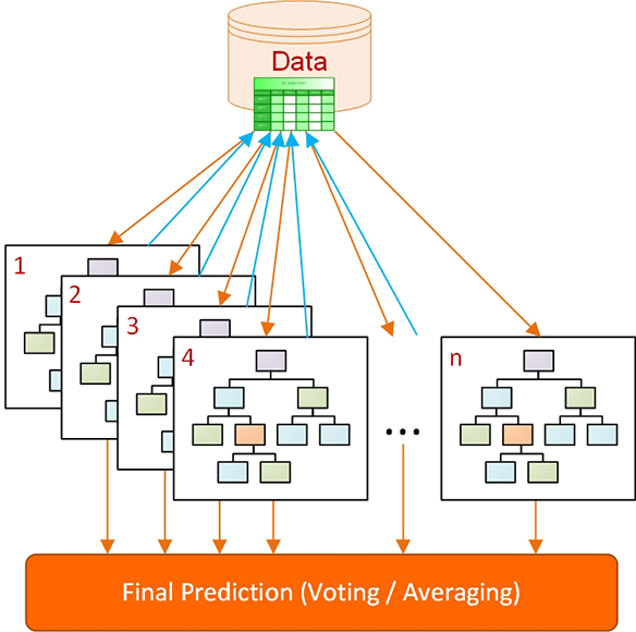
Figure 6.4 Boosting type ensembles for decision trees
Although they look quite similar in structure and purpose, bagging and boosting employ slightly different strategies to utilize the training data set and to achieve the goal of building the best possible prediction model ensemble. The two key differences between bagging and boosting are as follows. Bagging uses a bootstrap sample of the cases to build decision trees while boosting uses the complete training data set. While bagging creates independent, simple trees to ensemble, boosting creates dependent trees (each tree “learning” from the previous one to pay more attention to the incorrectly predicted cases) that collectively contributes to the final ensemble.
Boosting methods are designed to work with weak learners, that is, simple models; the component models in a boosted ensemble are simple models with high bias, though low variance. The improvement with boosting is better, as with bagging, when algorithms that are unstable predictors are used. Decision trees are most often used in boosted models. Naiïve Bayes is also used but with fewer improvements over a single model. Empirically speaking, m boosting typically produces better model accuracy than single decision trees, or even from bagging type ensembles.
Variants of Bagging and Boosting
Bagging and boosting were the first ensemble methods that appeared in predictive analytics software, primarily with decision tree algorithms. Since their introduction, many other approaches to building ensembles have been developed and made available particularly in open source software (both as part of open analytics platforms like KNIME and Orange, and as class libraries in R and Python). The most popular and successful [advanced] variants of bagging and boositg are Random Forest and Stochastic Gradient Boosting, respectively.
Random Forests
Random forests (RF) was first introduced by Breiman in 2000 (Breiman, 2000) as a modification to the simple bagging algorithm. As with bagging, the algorithm begins with bootstrap sampled data, and one decision tree is built from each bootstrap sample. Compared to simple bagging, there is, however, an important twist to the random forest algorithm: at each split in the tree, staring from the very first split, rather than considering all input variables as candidates, only a random subset of variables is considered. Hence, in random forest, the bootstrap sampling technique applies to both random selection of cases and random selection of feature (i.e., input variables).
The number of cases and the number of variables to consider, along with how many trees to construct are all parameter to decide in building random forest models. The common practice suggests that the default number of variables to consider as candidates at each split point should be the square-root of the total number of candidate inputs. For example, if there were 100 candidate inputs for the model, a random 10 inputs are candidates for each split. This also means that it is unlikely that the same inputs will be available for splits at parent and children nodes in a given tree, forcing the tree to find alternate ways to maximize the accuracy of subsequent splits in the tree. Therefore, there is an intentionally created two-fold diversity mechanism built into the tree construction process—random selection of cases and variables. Random forest models produce prediction outcomes that are usually more accurate than simple bagging and are often more accurate than simple boosting (i.e., AdaBoost).
Stochastic Gradient Boosting
The simple boosting algorithm, named AdaBoost, is only one of many boosting algorithms currently documented in the literature. In commercial software AdaBoost is still the most commonly used boosting technique, however, dozens of boosting variants can be found in the open source software packages. One interesting boosting algorithm that is recently gaining popularity due to its superior performance, is the Stochastic Gradient Boosting (SGB) algorithm created by Jerry Friedman at Stanford University. Then Friedman developed an advanced version of this algorithm (Friedman, 2001) that he called Multiple Additive Regression Trees (MART) and was later branded as TreeNet® by Salford Systems in its software tool. Like other boosting algorithms, the MART algorithm builds successive, simple trees and combines them additively. Typically, the simple trees are more than stumps and will contain up to six terminal nodes. Procedurally, after building the first tree, errors (also called residuals) are computed. The second tree and all subsequent trees then use residuals as the target variable. Subsequent trees identify patterns that relate inputs to small and large errors. Poor prediction of the errors results in large errors to predict in the next tree, and good predictions of the errors result in small errors to predict in the next tree. Typically, hundreds of trees are built, and the final predictions are an additive combination of the predictions that is, interestingly, a piecewise constant model because each tree is itself a piecewise constant model. However, one rarely notices because typically hundreds of trees are included in the ensemble (Abbott, 2014). The TreeNet algorithm, an example of stochastic gradient boosting, has won multiple data mining modeling competitions since its introduction and has proven to be an accurate predictor with the benefit that very little data cleaning is needed for the trees before modeling.
Stacking
Stacking (a.k.a. Stacked Generalization or Super Learner) is a part of heterogeneous ensemble methods. To some analytics professional, it may be the optimum ensemble technique but is also the least understood (and the most difficult to explain). Due to its two-step model training procedure, some thinks of it as an overly complicated ensemble modeling. Simply put, stacking creates an ensemble from a diverse group of strong learners. In the process, it interjects a metadata step called “super learner” or “meta learner”. These intermediate meta-classifiers are forecasting how accurately the primary classifiers have become and are used as the basis for adjustments and corrections (Vorhies, 2016). The process of stacking is figuratively illustrated in Figure 6.5.
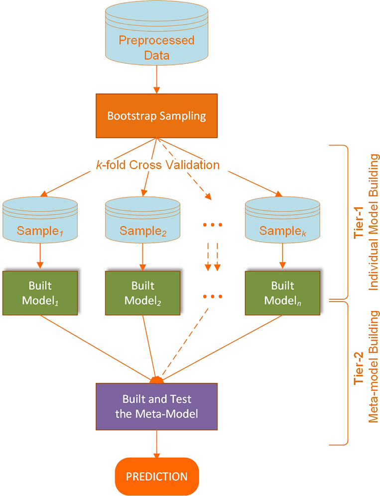
Figure 6.5 Stacking type model ensembles
As shown in Figure 6.5, in constructing stacking type model ensemble, a number of diverse strong classifiers are first trained using bootstrapped samples of the training data, creating Tier 1 classifiers (each optimized to its full potential for the best possible prediction outcomes). The outputs of the Tier 1 classifiers are then used to train a Tier 2 classifier (i.e., a meta-classifier) (Wolpert, 1992). The underlying idea is to learn whether training data have been properly learned. For example, if a particular classifier incorrectly learned a certain region of the feature space, and hence consistently misclassifies instances coming from that region, then the Tier 2 classifier may be able to learn this behavior, and along with the learned behaviors of other classifiers, it can correct such improper training. Cross validation type selection is typically used for training the Tier 1 classifiers—the entire training dataset is divided into k number of mutually exclusive subsets, and each Tier-1 classifier is first trained on (a different set of) k-1 subsets of the training data. Each classifier is then evaluated on the kth subset, which was not seen during training. The outputs of these classifiers on their pseudo-training blocks, along with the actual correct labels for those blocks constitute the training dataset for the Tier 2 classifier.
Information Fusion
As part of heterogeneous model ensembles, information fusion combines (fuses) the output (i.e., predictions) of different types of models such as decision trees, artificial neural networks, logistic regression, support vector machines, naïve Bayes, k-nearest neighbor, among other, and their variants. The difference between stacking and information fusion is the fact that in information fusion there is no “meta-modeling” or “super-learners.” It simply combines the outcomes of heterogeneous strong classifiers using simple or weighted voting (for classification) or simple or weighted averaging (for regression). Therefore, it is simpler and less computationally demanding than stacking. In the process of combining the outcomes of multiple models, either a simple voting (each model contributes equally, one vote) or a weighted combination of voting (each model is contributing based on its prediction accuracy—more accurate models are having higher weight value) can be used. Regardless of the combination method, this type of heterogeneous ensembles has been shown to be an invaluable addition to any data mining and predictive modeling projects. Figure 6.6 graphically illustrates the process of building information fusion type model ensembles.
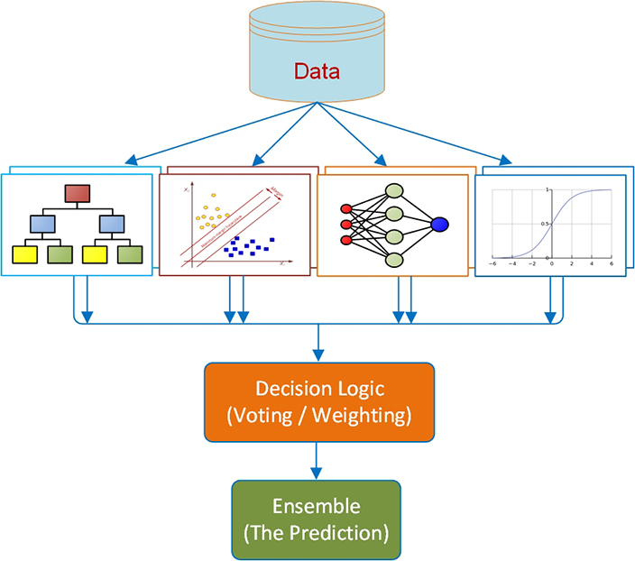
Figure 6.6 An illustration of building process for information fusion type model ensemble
Ensembles Are Not Perfect!
As a prospective data scientist, if you are asked to build a prediction model (or any other analytics model for that matter) you are expected to develop some of the popular model ensembles along with the standard individual models. If done properly, you will realize that ensembles are often more accurate and almost always more robust and reliable than the individual models. Although they seem like silver bullet, model ensembles are not without shortcomings, of which, following are the two most common ones:
Complexity
Model ensembles are more complex than individual models. Occam’s razor is a core principle many data scientists use, where the idea is that simpler models are more likely to generalize better, so it is better to reduce/regularize complexity, or in other words, simplify the models so that the inclusion of each term, coefficient, or split in a model is justified by its power of reducing the error at a sufficient amount. One way to quantify the relationship between accuracy and complexity is taken from information theory in the form of information theoretic criteria, such as the Akaike information criterion (AIC), the Bayesian information criterion (BIC), and Minimum Description Length (MDL). Traditionally statisticians, more recently data scientists, are using these criteria for variable selection in predictive modeling. Information theoretic criteria require a reduction in model error to justify additional model complexity. So the question is “do model ensembles violate Occam’s razor?” Ensembles, after all, are much more complex than single models. According to Abbott (2014), if the ensemble accuracy is better on held-out data than single models then the answer is “no” as long as we think about the complexity of a model in different terms—not just computational complexity but behavioral complexity. Therefore, we should not fear that adding computational complexity (more terms, splits, or weights) will necessarily increase complexity of models, because sometimes the ensemble will significantly reduce the behavioral complexity.
Transparency
The interpretation of ensembles can become quite difficult. If you build a random forest ensemble containing 200 trees, how do you describe why a prediction has a particular value? You can examine each of the trees individually, though this is clearly not practical. For this reason, ensembles are often considered black box models, meaning that what they do is not transparent to the modeler or domain expert. Although you can look at the split statistics (which variables are more often picked to split early in those 200 trees) to artificially judge the level of contribution (a psoudu veriable importance) each variable is contributing to the traned model ensemble. Compared to a single decision tree, this will still be too difficult and not as intuitive way to interpret how the model does. Another way to determine which inputs to the model are most important is to perform a sensitivity analysis.
In addition to complexity and transparency, model ensembles are also harder and computationally more expensive to built, and much more difficult to deploy. Table 5.9 shows the pros and cons of ensemble models as they compared to individual models.
Table 5.9 A brief list of pros and cons of model ensembles (as they are compared to individual models)

In summary, model ensembles are the new frontier for predictive modelers who are interested in accuracy, either by reducing errors in the models or by reducing the risk that the models will behave erratically. Evidence for this is clear from the dominance of ensembles in predictive analytics and data mining competitions: ensembles always win.
The good news for predictive modelers is that many techniques for building ensembles are built into software already. The most popular ensemble algorithms (bagging, boosting, stacking and their variants) are available in nearly every commercial or open source software tool. Building customized ensembles is also supported in many software products, whether based on a single algorithm or through a heterogeneous ensemble.
Ensembles aren’t appropriate for every solution—the applicability of ensembles is determined by the modeling objectives defined during business understanding and problem definition—but they should be part of every predictive modeler’s and data scientist’s modeling arsenal.
Bias-Variance Tradeoff in Predictive Analyztics
In predictive analytics, there is always a tradeoff between simplicity/parsimony and complexity, generalizability (capturing the signal) and overfitting (including the noise), predictive accuracy and explainability, overtraining/curve-fitting and undertraining, training error and validation error while developing machine learning models. The bias-variance tradeoff happens to the general concept that deals with these range of balancing acts. It is, in fact, a rather common concept discussed in statistics and machine learning that generally deals with the assessment of a trained predictive model in terms of its usefulness and accuracy. It is considered as a crucial issue to deal with in predictive modeling, data mining, machine learning, and supervised learning. Although the best model is achieved when both bias and variance is minimized, as the word “tradeoff” in the name implies, these two concepts (bias and variance) oppose each other—they do not go in the same direction; improving one worsens the other—and hence, a balancing act need to be performed. Finding the optimal combination of these two to achieve the best predictive model for a given problem and data combination is anything but a trivial process; often requiring consideration of best (or better) practices along with extensive experimentation and comparative analyses; even then, the obtained model cannot be confirmed as globally “optimal.”
What Is Bias and Variance?
Bias is the characterization of the training error—the difference between the model’s prediction output and the ground truth (i.e., the real/actual values) for a given prediction problem. A model with a high bias is the one that captures very little of the desired signal (i.e., patterns and relationships) in the training data, thereby produces an oversimplified/underfit model. As a result, such a model leads to high error values on both training and testing data.
Variance, on the other hand, is the characterization of the testing error—the variability of the model’s predictions for a given data set that characterizes the robustness of the prediction model. A model with a high variance is the one that captures not only the signal (i.e., generalized patterns and relationships) in the data but also the noise, thereby produces an overly complex/overfit model. As a result, such a model performs well on training data but does very poorly on the test data.
To graphically and intuitively illustrate the tradeoff between bias and variance, we often use a bullseye diagram, as in Figure 6.7. In this diagram, bias values are depicted on the y-axis and the variance values are depicted on the x-axis. For simplicity, the whole diagram is split into four quadrants (Q1 true Q4) in a two-dimensional Cartesian coordinate system along the dichotomized values of the x- and y-axis—namely, low and high. The simple interpretations of these quadrants are as follows:
• Q1: high bias, low variance. The predictions are consistent but are off-target/inaccurate (representing a consistently under-performing prediction model).
• Q2: high bias, high variance. The predictions are neither consistent nor accurate (representing an underperforming and inconsistent prediction model).
• Q3: low bias, low variance. The predictions are both consistent and accurate (representing the ideal prediction model).
• Q4: low bias, high variance. The predictions are inconsistent but somewhat accurate (representing a reasonably well performing but inconsistent prediction model).
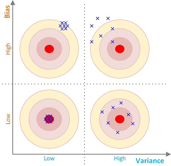
Figure 6.7 A bullseye diagram illustration of the bias-variance tradeoff
Overfitting versus Underfitting
The process of training of a predictive model is often characterized as “fitting” as in the case of “fitting a model to a given dataset.” Figure 6.8 shows the three levels of fitting/training/learning (i.e., overfitting, underfitting, and balanced-fitting) on a two-dimensional feature space. Overfitting (also called as overtraining) is the notion of making the model too specific to the training data), and by doing so, not only capturing the signal but also the noise in the dataset. As a result, the overtrained model (especially the highly parametrized model types like neural networks) will perform exceptionally well (at the level of “too good to be true”) on the training data and will do equally poorly on the test data. This phenomenon is also commonly characterized on the bias-variance-tradeoff continuum as low-bias high-variance outcome.
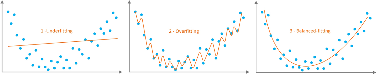
Figure 6.8 The three levels of fitting the model to the training data
On the other hand, underfitting (also called as undertraining) is the notion of leaving the model too generic, not completing the training (the learning process) from the training data (not capturing the signal inherent into the training data), and therefore, not performing as well as expected on the training data (or the testing data—although an undertrained model may perform equally well on the test data, because of its poor performance on the training data, such a performance may not be nearly sufficient for any practical purposes). Like overfitting but in reverse direction, this phenomenon is also commonly characterized on the bias-variance-tradeoff continuum as high-bias low-variance outcome.
What is desired for a predictive model is to avoid both overtrading and undertraining, and by doing so, achieve and optimal balance in fitting the model to the available taring data.
How to Determine the Optimal Level of Training
Most machine learning tools are formulated to learn from data in an iterative manner. With each iteration, the tool tries to incorporate more and more details deduced/inferred from the data in order to minimize the error. Since predictive models are at the core of supervised learning part of machine learning family of methods, during training/learning, they aimed to minimize the error (difference or delta), between the model output and the actual output. Each iteration focuses on reducing this error by adjusting the model parameters. For instance, in artificial neural networks, the learning process aims to minimize the difference between model output (the value of at the output layer) and the actual output of the data. Similarly, in decision tree induction, the learning process keeps growing the tree with new branches in order to purify the outputs at the leaf nodes (to achieve the perfect accuracy or matching).
Figure 6.9 graphically illustrates the change in the prediction error (and its reflection to the bias and variance curves/values) on the y-axis as the complexity of the model (and the training/learning process) progressively changes/evolves. As shown in the figure (the left-end of the x-axis), the simplest, least complex models characterized as the under-trained, under-learned, underfitted models, will have large error values (low prediction accuracy on the training), high-level of bias, and low-level of variance. The most complex models (the right-end of the x-axis), characterized as the over-trained, over-learned, overfitted models, will have very low error values (low prediction accuracy on the training data), low-level of bias, and high-level of variance.

Figure 6.9 The Nonlinear Relationship Between Error/Complexity and Bias/Variance.
Building a good prediction model requires us to find an optimal balance between the errors related to bias and variance. The optimal balance between the bias and variance can be determined by summing the error values that represents the two curves into a total error curve (a concave shaped curve), and then identifying/calculating the lowest point in the curve. This lowest point can be used to find the corresponding “optimal” values on complexity and the corresponding best achievable error value. The individual errors and the total error associated with each of the three curves in Figure 6.9 can mathematically be formulated as follows:

Error(x) is the sum of the three error terms: bias2, variance and the noise (i.e., the irreducible error). Irreducible error, as the name implies, cannot be reduced further by more training and employment of more sophisticating the model. It is considered as the noise in the model that we have to live with, which is usually the manifestation of missing (unrepresented) information in the variable space. In the real-world problems, which are complex and needs to be simplified via modeling assumptions, there will always be some degree of missing information (input variables), and hence, the model will never be perfectly or complete to produce zero noise.
Imbalanced Data Problem in Predictive Analytics
Developing prediction models using imbalanced datasets is one of the most critical challenges in the field of data mining and decision analytics. A dataset is called imbalanced when the distribution of different classes in the target variable are significantly dissimilar. For instance, in the case of binary classification problem in medical testing, the data may have many more examples that belong to one class (e.g., negative examples) compared to the other class (positive examples). Usually, we call the class with fewer examples the minority class, and the class with more examples the majority class. Although most of the discussion on imbalanced data problem centers around the binary classification problems, the phenomenon also applies to multi-class classification problems as well as the problems that deal with numerical target variables (i.e., regression or estimation type prediction problems). Decision modeling based on imbalanced datasets is quite common in real-world problems, including medical diagnosis, fraud detection, churn analysis, email spam identification, outlier detection, bankruptcy prediction, network intrusion detection, among other.
The issues related to the imbalances data problem is especially obvious while developing clinical decision support systems where the cases with a rare disease would usually constitute a very small proportion of the total patient population. For instance, one of our earlier study involved in the development of a clinical decision support system for diagnosing diabetic retinopathy patients using only a small set of diabetes test results and patient demographic information (contained within the EHR database). In this dataset—a population of several hundred thousand diabetic patients—only about 5% of the patients had the diabetic retinopathy and the remaining 95% did not have the disease (Piri et al., 2017). Similarly, and perhaps a less severely imbalanced data problem was dealt within a decision support system we have developed for the educational institutions (i.e., educational decision support system). The main goal of the system was to identify, explain, and mitigate freshmen student attrition (Thammasiri et al., 2014) at a higher education institution. In this student attrition prediction problem, we had a dataset that contained about four times more negative samples (freshmen students that did not attrite/dropped-out) compared to the positive samples (freshmen students that did attrite/dropped-out). Figure 6.10 graphically illustrates the data imbalance situation dealt with while developing this system. As can be seen on the right side of the figure (the model assessment pane), the imbalanced data produced very high predictive accuracy on the majority class but performed very poorly on the minority class, while balanced data produced significantly better, near equal prediction accuracy for both minority and majority classes. Although the overall accuracy achieved with imbalanced dataset seems to be scientifically higher, this is a rather deceptive perception, which is often characterized as “fool’s gold” in data mining literature. In summary, a balanced dataset allows machine learning techniques to produce reasonably high prediction accuracy for both classes.
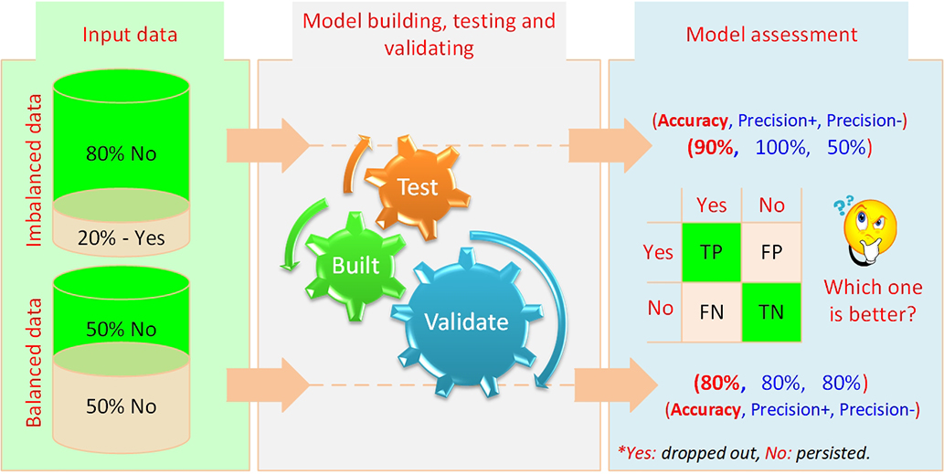
Figure 6.10 A Graphical Depiction of the Class Imbalance Problem.
But why does imbalanced dataset lead to poor prediction outcomes? Machine learning methods learns from the training data in somewhat of a similar manner that humans learn from their experiences. That is, in humans (and perhaps in most animals as well), memory and recall is largely determined by repeated events and experiences. Frequently observed experiences lead to more permanent and vivid memories that leads to easier and more accurate recall and recognitions. In contrary, the less observed experiences are often oversight or simply ignored in the process, and hence are often not accurately recalled when needed. In machine learning, a similar learning process takes place, where the method produces biased predictive models that focuses on the majority class patterns while conveniently ignoring the minority class specifics.
The Methods to Solve the Imbalanced Data Problem
There are various approaches to mitigate the imbalanced data problem and thereby improve the performance of a given predictive model. A simple taxonomy of the methods used to handle the imbalanced data problem is shown in Figure 6.11. Although they may differ in level of algorithmic sophistication, the goal of all of these methods is to make sure the prediction method (or the underlying algorithm) pays near-equal/fair attention to patterns presented by all classes, majority, minority and anything in between. While some of these methods try to solve the imbalanced data problem by simply manipulating the distribution of the classes in the training data, others try to manipulate the learning process by adjusting the underlying algorithm or adjusting the cost of performance to favor the accurate prediction of the minority class.

Figure 6.11 A Taxonomy of Methods Used to Handle the Imbalanced Data Problem
Data sampling methods—the most widely used class of methods in data science and machine learning because of their ease of understanding, formulation, and implementation—are those that either increase the number of minority examples by generating additional examples (collectively called as oversampling methods) or decrease the number of majority examples by removing some of them (usually called as Undersampling methods). Oversampling methods increase the number of examples in the minority class by one of two ways: (1) replicating the examples in the minority class until the they are equal to the number of examples in the majority class (via a simple copy-paste or a bootstrapping type random sampling), or (2) syntactically creating new examples that ar not the same but are very similar to the samples in the minority class. A popular technique called SMOTE (Synthetic Minority Oversampling TEchnique) syntactically creates similar minority class examples using k-nearest neighbor algorithm (as the similarity measure to create the syntactic examples to increases the number of examples in the minority class. SMOTE works quite well with datasets that are dominated by genuinely numerical input variables, and inversely, does a very poor job on the datasets that are dominated by categorical/nominal variables. There have been numerous attempts to create variants of SMOTE algorithms that handles the shortcoming of the original algorithm. Undersampling, on the other hand, keeps the minority class examples as is, and randomly samples equal number of examples from the majority class. That is, some of the majority class examples will be excluded from the training dataset. The random selection can be with (i.e., bootstrapping) or out without replacement.
Another class of methods used to handle class imbalance problem focuses on the misclassification cost. While data sampling methods focus on balancing the data prior to the learning/training process this class of methods focus on adjustment to the cost of classification performance. Specifically, this class of methods assigns different misclassification costs to various classes based on the severity of the imbalance nature of the data, and therefore, is called cost sensitive methods. In practice, these methods aim to either adjust the classification threshold or assigns disproportional cost to classes to enhance the focus on the minority class.
Another stream of methods to handle the imbalanced data problem focuses on algorithmic adjustments to a variety of classification algorithms. Although the goal of all of these adjusted classification algorithms are the same (i.e., mitigating the effect of imbalanced data), the specific methods used by each algorithm uses to achieve this goal differs significantly. One of the most studied class of methods that benefited from this type of mitigation is of the support vector machine and its variants. For example, in a recent research project, we developed a novel synthetic informative minority over-sampling (SIMO) algorithm that employs support vector machine to enhance the learning from imbalanced dataset by creating syntactic examples of the minority class near the support vectors (the hard to classify regions in the multi-dimensional feature space) (Piri et al., 2018).
The one-class method has also been used by the machine learning community to address class imbalance problem. The general idea behind the one-class method is to focus on only one class label at a time. That is, the training data samples are all from a single class label (e.g., all positive or all negative samples) to learn only the specific characteristics of that class. Because this method focuses on recognizing and predictand only one class (as opposed to the case in ordinary classification methods where models are developed to discern/differentiate between two or more classes), this approach is often called “recognition-based” while the latter is called as the “discrimination-based” method. Because the main idea behind this method is to make the underlying model specific to the characteristics of one class, and recognizes everything else not belonging to that class, it utilize the following three unification/homogenization approaches: (1) density-based characterization, (2) boundary determination, and (3) reconstruction/evolution-based specification. These approaches borrow their conceptual depiction and related functionalities from, and hence can be thought of the extensions of, the clustering algorithms such as k-means, k-medoids, k-centers, and self-organizing maps.
Some of the latest methods to handle the imbalanced data problem emerged from the field of ensemble methods. As opposed to using a single prediction model, this type of models utilizes a number of either the same type methods (homogeneous ensembles) or different (heterogeneous ensembles) prediction model outcomes to mitigate the negative effects of the imbalanced data. Variants of both bagging and boosting type ensemble methods are proposed as solutions to class imbalance problems where in the case bagging the random sampling is adjusted to favor the minority class and in the case of boosting the weights for the minority class samples are adjusted disproportionally. Active learning—a methodology that learns iteratively in a piecewise manner—is also being explored as a way to handle the class imbalance problem.
Despite the fact that there have been numerous efforts to address the class imbalance problem in machine learning community, the current state of the art is still limited to heuristic solutions and ad hoc methodologies. There still is a lack of universally accepted theories, methodologies, and best practices. Although most studies claim to have developed data balancing methodologies that improved the prediction accuracy on the minority class, a significant number of studies also concluded that these methodologies worsen the prediction accuracy on the majority class and on the overall classification accuracy. The ongoing research is still seeking to answer the question like “can there be a single universal methodology that produces better prediction results?” or “can there be a methodology that can prescribe the best data balancing algorithm for a given machine learning method and the specifics of the data on hand?”
Explainability of Machine Learning Models for Predictive Analytics
In predictive analytics (and machine learning), there has been a trade-off between model complexity and model performance—more complex the machine learning models (e.g., deep neural networks, random forest, and gradient boosted machines) more accurate is the prediction outcomes. As the model gets simpler (move towards more parsimony), less predictive performance is observed, but at the same time, more interpretable and transparent the model becomes. The seminal research paper by Ribiero et al. (2016) entitled “Why Should I Trust You,” appropriately highlights the issue with machine learning models and their infamous nature of being black boxes. With the new and enhanced interest in machine learning methods, especially since the advent of model ensembles and deep learning, model interpretability has become a fast-growing field of research; nowadays this trend is appropriately called as Explainable AI and Human Interpretable Machine Learning.
As you have seen in this book, predictive analytics methods and their underlaying machine learning algorithms are really good at capturing complex relationships between input and output variables (producing very accurate prediction models), but are not nearly as good at explaining how they do what they do (i.e., model transparency / model explainability). In order to mitigate this deficiency (also called the “black-box syndrome”), machine learning community proposed several methods, most of which are characterized as sensitivity analysis. Some of these methods are global (providing explanation based on average score of all data samples) and some are local (providing single sample level explanations). In the context of predictive modeling, sensitivity analysis usually refers to an exclusive experimentation process designed and executed to discover the cause and effect relationship between the input variables and output variable. Some of the variable importance methods are model/algorithm specific (i.e., applied to decision trees, neural networks, or random forest) and some are model/algorithm agnostic (i.e., applied to any and every predictive model). Here are the most commonly used variable importance methods employed in machine learning and predictive modeling:
1. Developing and observing a well-trained decision tree model to see the relative discernibility of the input variables—closer to the root of the tree a variable is used to slit, greater is its importance/relative-contribution to the prediction model.
2. Developing and observing a rich and large random forest model and assessing the variable split statistics. If the ratio of a given variable’s selection into candidate counts (i.e., number of times a variable selected as the level-0 splitter divided by number of time it was picked randomly as one of split candidates) is larger, then its importance/relative-contribution is also greater. This process can be extended to the tops three layers of the trees to generate a weights average of the split statistics and can be used as a measure of variable importance for random forest models.
3. Sensitivity analysis based on input value perturbation, where the input variables are gradually and systematically changed/perturbed one at a time and the relative change in the output is observed—larger the change in the output, greater the importance of the perturbed variable. This method is often used in trained feed-forward neural network modeling where all of the input variables are numeric and standardized/normalized.
4. Sensitivity analysis based on leave-one-out methodology. This method can be applied to any type of predictive analytics method (i.e., predictive model agnostic). Because of its general applicability and ease of implementation, this sensitivity analysis method is used in several commercial and free/open source analytics tools as the default functionality, and therefore is further explained below.
5. Sensitivity analysis based on developing a surrogate model to assess the variable importance of a single record/sample using LIME of SHAP methodologies. While the previous methods are considered global interpreters, LIME and SHAP are called local because they explain the importance of the variables at the sample level (as opposed to the average of all samples). Because of the increased interest in these latest methods, they (LIME and SHAP) will be explained below.
Sensitivity Analysis Based on Leave-One-Out Methodology
The sensitivity analysis based on leave-one-out methodology relies on the experimental process of systematically removing input variables, one at a time, from the input variable set, developing and testing a model, and observing the impact of the absence of this variable on the predictive performance of the machine learning model. Specifically, first, the model is trained and tested (often using a k-fold cross validation) with all input variables, and the best predictive accuracy is recorded as the baseline. Then, the same model with the exact same settings is trained and tested with all but one input variable, and the best prediction accuracy is recorded, and this process is repeated as many times as the number of variables, each time omitting/excluding a different input variable. Then the degradation from the baseline is measured for the omission of each variable, and these measures are used to create a tabular and graphical illustration of the variable importance as shown in Figure 6.12.
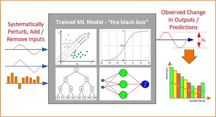
Figure 6.12 A graphical depiction of the sensitivity analysis process
This sensitivity analysis method can be used for any predictive analytics and machine learning method, and historically, it has often been often used for support vector machines, decision trees, logistic regression as well as for artificial neural networks. Saltelli (2002), in his sensitivity analysis book, formalized the algebraic representation of this measurement process with the following equation.
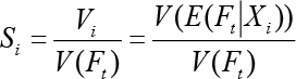
In this equation, the denominator, V(Ft), refers to the variance in the output variable. In the numerator, V(E(Ft∣Xi)), E is the expectation operator to calls for an integral over parameter Xi; that is, inclusive of all input variables except Xi, the V, the variance operator applies a further integral over Xi. The variable contribution (i.e., importance), represented as Si, for the ith variable, is calculated as the normalized sensitivity measure. In a later study, Saltelli et al (2004) proved that this equation is the most probable measure of model sensitivity that is capable of ranking input variables (i.e., the predictors) in the order of importance for any combination of interactions including the non-orthogonal relationships amongst the input variables.
Using this method of sensitivity analysis may produces slightly different importance measures for different model types for the same dataset. In such situation, we can either select and use the variable importance measured of the most predictive model type while ignoring the ones generated by the other model-types, or we can use some type combination (i.e., ensemble) of all importance measures produced by all model types. In order to properly combine the sensitivity analysis results for all prediction model types, we can use an information fusion-based methodology—a weighted average where the weights are determined based on the prediction power of the individual model types. Particularly, by modifying the above equation in such a way that the sensitivity measure of an input variable n obtained based on the information combined (i.e., fused) from m number of prediction model types. Following equation represents this waited summation function.

In this equation ωi represents the normalized contribution/weight for each prediction model where the level of contribution/weight of a model is calculated as a function of its relative predictive power—larger the prediction power (i.e., accuracy) greater the value of ω.
Local Interpretability with LIME and SHAP
In linear regression models, beta coefficients explain the prediction for all the data points (i.e., if a variable value increases by one unit, prediction value increases by beta for every data point). This is commonly called as global interpretability. In a causal modeling, this is called average causal analysis (Nayak, 2019). However, this does not specifically explain individual differences—the effect of variable values for rejecting the loan application of one applicant could be different than another. This is local often called local interpretability which is the explanation for an individual data point or local subsection of the joint distribution of independent variables. LIME and SHAP are the two recent and popular methods that aims to provide local explainability by building surrogate models to the black-box. They tweak the input slightly (like we do in sensitivity analysis) and test the changes in prediction through a surrogate model representation (Figure 6.13). Since these surrogate models still treat the machine learning models as a black box, these methodologies are considered as model agnostic.
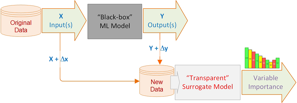
Figure 6.13 From global black-box model to local surrogate model for variable importance
Local Interpretable Model-Agnostic Explanations (LIME) is a relatively new variable assessment method developed to explains the prediction of any prediction model (i.e., classifier) in a human interpretable manner by developing/learning a surrogate model locally based on the specifics of the prediction (the predicted case/sample). The main idea behind LIME is to simulate the relationships between inputs and outputs of a complex machine learning model by developing a surrogate (similar but much simpler and explainable) model for explaining the prediction results of a single record (i.e., a specific customer). To do so, the surrogate model utilizes a sample of synthetically generated records closely resembling the actual predicted record itself. What have made LIME a popular technique includes it being model agnostic (works with any type of prediction model), ability to generate human interpretable outcomes, providing the explanation at the local (single record) level, being additive (the sum of importance values of all the variables for a data point is equal to the final prediction), and being a computationally very efficient algorithm. More on LIME and its algorithmic details can be found in Ribeiro et al. (2016).
Shapley Additive Explanations (SHAP) is another recently proposed technique for model interpretation. It is widely considered as the best local model interpretation technique, superior to LIME in several dimensions. Although SHAP employs a similar concept to LIME, it provides theoretical guarantees based on the game theory concept of Shapley values; it is capable of capturing and representing complex relationships at the local level beyond just linear relationships, and produces more accurate, robust, and reliable interpretation outcomes. SHAP can also be used effectively for variable selection—we can select a subset of the variables with higher variable importance, drop other variables (if we want to reduce the number of variables); because of its consistency property, the order of variable importance do not change, hence less important variables can be ignored. More detailed on SHAP can be found in Lundberg and Lee (2017).
Which Technique Is the Best?
As is the case almost always, there is no magic answer or solution to this question that applies to all problems and situations. If you are interested in model agnostic global explainability, perhaps the leave-one-out type sensitivity analysis could be used. If a model specific interpretation is desired, then the appropriate sensitivity analysis for the specific model type could be utilized. If you desire local interpretation, then either LIME of SHAP can be used; out of these two, SHAP is considered as a better method but it is computationally more expensive than LIME. If a quick explanation at the single record level is needed for a large and complex problem space, perhaps LIME could be the method of choice.
Application Case: To Imprison or Not to Imprison—A Predictive Analytics-Based Decision Support System for Drug Courts
Analytics has been used by many businesses, organizations, and government agencies to learn from past experiences to more effectively and efficiently use their limited resources towards achieving their goals and objectives. Despite all the promises of analytics, however, its multidimensional and multidisciplinary nature can sometimes disserve its proper, full-fledged application. This is particularly true for the use of predictive analytics in several social science disciplines, as these domains are traditionally dominated by descriptive analytics (causal-explanatory statistical modeling) and may not have an easy access to the set of skills required to build predictive analytics models. A review of the extant literature shows that drug court is one such area. While many researchers have studied this initiative, its requirements, and its outcomes from a descriptive analytics perspective, there currently is a dearth of a predictive analytics model that can accurately and appropriately predict who would (or would not) graduate from these programs. To fill this gap and to help authorities better manage the resources and improve the outcomes, this study aims to develop and compare several predictive analytics models (both single models and ensembles) to identify who would graduate from these treatment programs.
Ten years after President Nixon first declared a “war on drugs,” President Reagan signed an executive order leading to stricter drug enforcement, stating, “We’re taking down the surrender flag that has flown over so many drug efforts; we are running up a battle flag.” The reinforcement of the “war on drugs” resulted in an unprecedented ten-fold surge in the number of citizens incarcerated for drug offences during the following two decades. The skyrocketed drug cases inundated court dockets, overloaded the criminal justice system, and overcrowded the prisons. The abundance of drug-related caseloads, aggravated by their longer processing time in contrast to most other felonies, imposed tremendous costs on state and federal departments of justice. Regarding the increased demand, court systems started to look for innovative ways to accelerate the inquest of drug-related cases. Perhaps analytics driven decision support systems are the solution to the problem. To support this claim, the current study sets out to build and compare several predictive models that use a large sample of drug courts data across different locations to predict who is more likely to complete the treatment successfully. We believe this endeavour can reduce the costs that the criminal justice system and local communities undergo in the course of these initiatives.
Methodology
The methodology we used in this effort included a multi-step process that aimed at employing predictive analytics methods in a social science context. The first step of this process, which focused on understanding the problem domain and the need to conduct this study, was presented in the previous section. For the following steps of the process, we employed a structured and systematic approach to develop and evaluate a set of predictive models using a large and feature-rich real-world data set. These steps included data understanding, data preprocessing, model building, and model evaluation and are reviewed in this section. Our approach also involved multiple iterations of experimentations and numerous modifications to improve individual tasks and to optimize the modeling parameters to achieve the best possible outcomes. A pictorial depiction of our methodology is given in Figure 6.14.
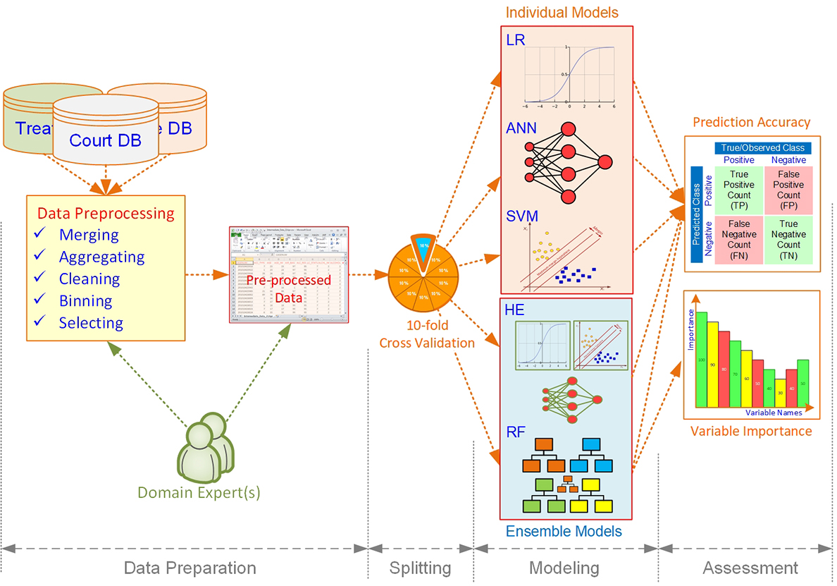
Figure 6.14 Research methodology depicted as a workflow
Results
A summary of the models’ performances based on accuracy, sensitivity, specificity, and AUC is presented in Table 6.10. As the results show, RF has the best classification accuracy and the greatest AUC among the models. The HE model closely follows RF and SVM, ANN, and LR rank third to last based on their classification performances. RF also has the highest specificity and the second highest sensitivity. Sensitivity in the context of this study is an indicator of a model’s ability in correctly predicting the outcome for successful participants. Specificity, on the other hand, determines how a model performs in predicting the end results for those who do not complete the treatment. Consequently, we can conclude that RF outperforms other models for the drug courts data set used in this study.
Table 6.10. Performance of predictive models using 10-fold cross-validation on the balanced data set
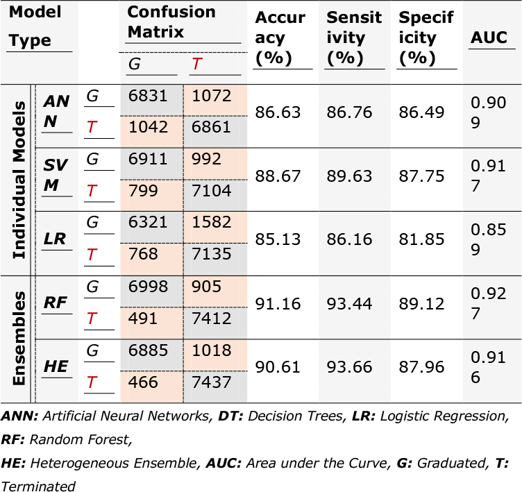
Although the RF model performs better than the other models in general, it falls second to the HE model in the number of false negative predictions. Similarly, the HE model has a slightly better performance in true negative predictions. False positive predictions represent participants who were terminated from the treatment, but the models mistakenly classified them as successful graduates. False negatives pertain to individuals that graduated, but the models predicted them as dropouts. False positive predictions are synonymous with increased costs and opportunity losses, whereas false negatives carry social impacts. Spending resources on those offenders who would recidivate at some point in time during the treatment, and hence, be terminated from the program takes the opportunity of participating in the treatment from a number of (potentially successful) prospective offenders. Conspicuously, depriving potentially successful offenders from the treatment is against the initial objective of drug courts in reintegrating nonviolent offenders into their communities.
In summary, traditional causal-explanatory statistical modeling, or descriptive analytics, uses statistical inference and significance levels to test and evaluate the explanatory power of hypothesized underlying models or to investigate the association between variables retrospectively. Although a legitimate approach for understanding the relationships within the data used to build the model, descriptive analytics falls short in predicting outcomes for prospective observations. In other words, partial explanatory power does not imply predictive power and predictive analytics is a must for building empirical models that predict well. Therefore, relying on the findings of this study, application of predictive analytics (rather than the sole use of descriptive analytics) to predict the outcomes of drug courts is well-grounded.
Summary
Predictive analytics is still developing with novel methods and methodologies. Idea behind these developments is to address the shortcomings of the exiting techniques, to create more accurate and more explainable models. To that end, this chapter covers a few recent advances in predictive analytics, namely model ensembles, bias-variance tradeoff, imbalance data problems, and explainable AI/machine learning. While the first three focus on building more accurate and unbiased predictive models, the last one (i.e., explainable AI/machine learning) focuses on making the black-box models transparent (may be not completely transparent but at least partially transparent) so that there model can be used in domains where explainability is one of the required characteristics from a prediction model.
References
Abbott, D. (2014). Applied predictive analytics: Principles and techniques for the professional data analyst. John Wiley & Sons. Hoboken, New Jersey.
Breiman, L. (1996). Bagging predictors. Machine learning, 24(2), 123-140.
Freund, Y. and Schapire, R.E. (1996). Experiments with a new boosting algorithm. In Machine Learning: Proceedings of the Thirteenth International Conference, 148–156.
Friedman, J. H. (2001). Greedy function approximation: a gradient boosting machine. Annals of Statistics, 1189-1232.
He, H., & Ma, Y. (Eds.). (2013). Imbalanced learning: foundations, algorithms, and applications. John Wiley & Sons.
Lundberg, S. M., & Lee, S. I. (2017). A unified approach to interpreting model predictions. In Advances in Neural Information Processing Systems, 4765-4774.
Nayak, A. (2019). Idea Behind LIME and SHAP, available at https://towardsdatascience.com/idea-behind-lime-and-shap-b603d35d34eb (Accessed July 2020).
Piri, S., Delen, D., & Liu, T. (2018). A synthetic informative minority over-sampling (SIMO) algorithm leveraging support vector machine to enhance learning from imbalanced datasets. Decision Support Systems, 106, 15-29.
Piri, S., Delen, D., Liu, T., & Zolbanin, H. M. (2017). A data analytics approach to building a clinical decision support system for diabetic retinopathy: Developing and deploying a model ensemble. Decision Support Systems, 101, 12-27.
Ribeiro, M. T., Singh, S., & Guestrin, C. (2016, August). “ Why should I trust you?” Explaining the predictions of any classifier. In the Proceedings of the 22nd ACM SIGKDD international conference on knowledge discovery and data mining, 1135-1144.
Sarkar, D. (2018). The Importance of Human Interpretable Machine Learning, available at https://towardsdatascience.com/human-interpretable-machine-learning-part-1-the-need-and-importance-of-model-interpretation-2ed758f5f476 (Accessed July 2020).
Seni, G., & Elder, J. F. (2010). Ensemble methods in data mining: improving accuracy through combining predictions. Synthesis Lectures on Data Mining and Knowledge Discovery, 2(1), 1-126.
Surowiecki, J. (2006). The Wisdom of Crowds. Penguin Random House publishing. New York, NY.
Thammasiri, D., Delen, D., Meesad, P., & Kasap, N. (2014). A critical assessment of imbalanced class distribution problem: The case of predicting freshmen student attrition. Expert Systems with Applications, 41(2), 321-330.
Vorhies, W. (2016). Want to Win Competitions? Pay Attention to Your Ensembles. Data Science Central Web Portal at www.datasciencecentral.com/profiles/blogs/want-to-win-at-kaggle-pay-attention-to-your-ensembles (accessed July 2018).
Wolpert, D. (1992). Stacked Generalization. Neural Networks, 5(2), 241-260, 1992.