Chapter 9
Deep Learning and Cognitive Computing
As you will see in this chapter, artificial intelligence (AI) in general and the methods of machine learning in specific are evolving and advancing rapidly. The use of large digitized data sources (both structured and unstructured) from both inside and outside the organization, along with the advanced computing systems (software and hardware combinations), has paved the way toward developing smart solutions to complex problems that were thought to be unsolvable just a few years ago. Deep learning and cognitive computing (as the ramifications of the cutting edge in AI systems) are helping enterprises to make accurate and timely decisions by harnessing the rapidly expanding Big Data resources. As witnessed in academia and in industry, these new generation of AI systems are capable of solving problems in a significantly different manner, producing results that are much better than their older counterparts. In the domain of fraud detection, for instance, traditional methods have always been marginally useful, having higher than desired false positive rates and causing unnecessary investigations and thereby dissatisfaction for their customers. As the good-old difficult problems, such as fraud detection, are resurfaces, reimagined, and redesigned, AI technologies like deep learning are making them solvable with a high level of accuracy and applicability.
Introduction to Deep Learning
About a decade ago, conversing with an electronic device (in human language, intelligently) would have been unconceivable, something that could only be seen in SciFi movies. Today, however, thanks to the advances in AI methods and technologies, almost everyone has experienced this unthinkable phenomenon. You probably have already asked Siri or Google Assistant several times to dial a number from your phone address book or to find an address and give you the specific directions while you were driving. Sometimes when you were bored in the afternoon, you may have asked the Google Home or Amazon’s Alexa to play some music in your favorite genre on the device or your TV. You might have been surprised at times when you uploaded a group photo of your friends on Facebook and observed its tagging suggestions where the name tags often exactly match your friends’ faces in the picture. Translating a manuscript from a foreign language does not require hours of struggling with a dictionary; it is as easy as taking a picture of that manuscript in the Google Translate mobile app and giving it a fraction of a second. These are only a few of the many, ever-increasing applications of deep learning that have promised to make the life easier for people.
Deep learning, as the newest and perhaps at this moment the most popular member of the AI and machine-learning family, has a goal similar to those of the other machine-learning methods that came before it: mimic the thought process of humans—using mathematical algorithms to learn from data pretty much the same way that humans learn. So, what is really different (and advanced) in deep learning? Here is the most commonly pronounced differentiating characteristic of deep learning over the traditional machine learning. The performance of traditional machine-learning algorithms such as decision trees, support vector machines, logistic regression, and neural networks relies heavily on the representation of the data. That is, only if we (analytics professionals or data scientists) provide those traditional machine learning algorithms with relevant and sufficient pieces of information (a.k.a. features) in proper format are they able to “learn” the patterns and thereby perform their prediction (classification or estimation), clustering, or association tasks with an acceptable level of accuracy. In other words, these algorithms need humans to manually identify and derive features that are theoretically and/or logically relevant to the objectives of the problem on hand and feed these features into the algorithm in a proper format. For example, in order to use a decision tree to predict whether a given customer will return (or churn), the marketing manager needs to provide the algorithm with information such as the customer’s socioeconomic characteristics such as income, occupation, educational level, and so on (along with demographic and historical interactions/transactions with the company). But the algorithm itself is not able to define such socioeconomic characteristics and extract such features, for instance, from survey forms completed by the customer or obtained from social media.
While such a structured, human-mediated machine-learning approach has been working fine for rather abstract and formal tasks, it is extremely challenging to have the approach work for some informal, yet seemingly easy (to humans), tasks such as face identification or speech recognition since such tasks require a great deal of knowledge about the world (Goodfellow et al., 2016). It is not straightforward, for instance, to train a machine-learning algorithm to accurately recognize the real meaning of a sentence spoken by a person just by manually providing it with a number of grammatical or semantic features. Accomplishing such a task requires a “deep” knowledge about the world that is not easy to formalize and explicitly present. What deep learning has added to the classic machine-learning methods is in fact the ability to automatically acquire the knowledge required to accomplish such informal tasks and consequently extract some advanced features that contribute to the superior system performance.
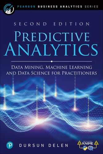
To develop and intimate understanding of deep learning, one should learn where it fits in the big picture of all other AI family of methods. A simple hierarchical relationship diagram, or a taxonomy-like representation, may in fact provide such a holistic understanding. In an attempt to do this, Goodfellow and his colleagues (2016) categorized deep learning as part of the representation learning family of methods. Representation learning techniques entails one type of machine learning (which is also a part of AI) in which the emphasis is on learning and discovering features by the system in addition to discovering the mapping from those features to the output/target. Figure 9.1 uses a Venn diagram to illustrate the placement of deep learning within the overarching family of AI-based learning methods.
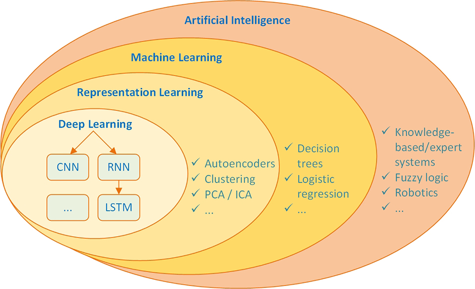
Figure 9.1 A Venn Diagram Showing the Placement of Deep Learning Within the Overarching AI-Based Learning Methods.
Figure 9.2 highlights the differences in the steps/tasks that need to be performed when building a typical deep learning model versus the steps/tasks performed when building models with classic machine-learning algorithms. As shown in the top two workflows, knowledge-based systems and classic machine-learning methods require data scientists to manually create the features (i.e., the representation) to achieve the desired output. The bottom most workflows show that deep learning enables the computer to derive some complex features from simple concepts that would be very effort intensive (or perhaps impossible in some problem situations) to be discovered by humans manually, and then it maps those advanced features to the desired output.
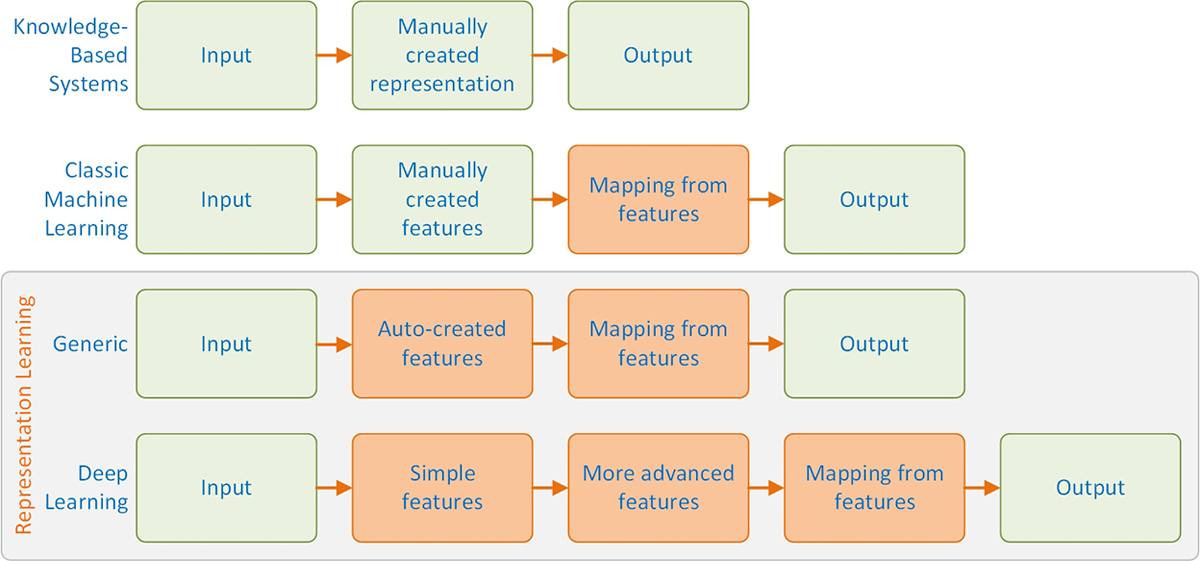
Figure 9.2 Illustration of the Key Differences Between Classic Machine-Learning Methods and Representation Learning/Deep Learning (shaded boxes indicate components that are able to learn directly from data).
From a methodological viewpoint, although deep learning is generally believed to be a new area in machine learning, its initial idea goes back to late 1980s, just a few decades after the emergence of artificial neural networks when LeCun et al. (1989) published an article about applying backpropagation networks for recognizing handwritten ZIP codes. In fact, as it is being practiced today, deep learning seems to be nothing but an extension of neural networks with the idea that deep learning is able to deal with more complicated tasks with a higher level of sophistication by employing many layers of connected neurons along with much larger data sets to automatically characterized variables and solve the problems but only at the expense of a great deal of computational effort. This very high computational requirement and the need for very large data sets were the two main reasons why the initial idea had to wait more than two decades until some advanced computational and technological infrastructure emerged for deep learning’s practical realization. Although the scale of neural networks has dramatically increased in the past decade by the advancement of related technologies, it is still estimated that having artificial deep neural networks with the comparable number of neurons and level of complexity existing in the human brain will take several more decades.
In addition to the computer infrastructures, as mentioned, the availability of large and feature-rich digitized data sets was another key reason for the development of successful deep learning applications in recent years. Obtaining good performance from a deep learning algorithm used to be a very difficult task that required extensive skills, experience, and in-depth understanding to design task specific networks, and therefore, not many were able to develop deep learning for practical and/or research purposes. Large training data sets, however, have greatly compensated for the lack of intimate knowledge and reduced the level of skill needed for implementing deep neural networks. Nevertheless, although the size of available data sets has exponentially increased in the recent years, a great challenge, especially for supervised learning of deep networks, is now the labeling of the cases in these huge data sets. As a result, a great deal of research is ongoing, focusing on how we can take advantage of large quantities of unlabeled data for semisupervised or unsupervised learning or how we can develop methods to label examples in bulk in a reasonable time.
The following section of this chapter provides a general introduction to neural networks from where deep learning has originated. Following the overview of these “shallow” neural networks, the chapter introduces different types of deep learning architectures and how they work, some common applications of these deep learning architectures, and some popular computer frameworks to use in implementing deep learning in practice. Since, as mentioned, the basics of deep learning are the same as those of artificial neural networks, in the following section, we provide a brief coverage of the neural network architecture (namely, multi-layered perceptron [MLP] type neural networks, which was omitted in the neural network section in Chapter 5 because it was to be covered here) to focus on their mathematical principles and then explain how the various types of deep learning architectures/approaches were derived from these foundations.
Basics of “Shallow” Neural Networks
Artificial neural networks are essentially simplified abstractions of the human brain and its complex biological networks of neurons. The human brain has a set of billions of interconnected neurons that facilitate our thinking, learning, and understanding of the world around us. Theoretically speaking, learning is nothing but the establishment and adaptation of new or existing inter-neuron connections. In the artificial neural networks, however, neurons are processing units (also called processing elements [PEs]) that perform a set of predefined mathematical operations on the numerical values coming from the input variables or from the other neuron outputs to create and push out its own outputs. Figure 9.3 shows a schematic representation of a single-input and single-output neuron (more accurately, the processing element in artificial neural networks).
Figure 9.3 General Single-Input Artificial Neuron Representation
In this figure, p represents a numerical input. Each input goes into the neuron with an adjustable weight w and a bias term b. A multiplication weight function applies the weight to the input, and a net input function shown by > adds the bias term to the weighted input z. The output of the net input function (n, known as the net input) then goes through another function called the transfer (a.k.a. activation) function (shown by f) for conversion and the production of the actual output a. In other words:
a = f (wp + b)
A numerical example: if w = 2, p = 3, and b = –1, then a = f(2*3 – 1) = f(5).
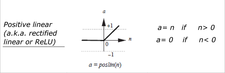
Various types of transfer functions are commonly used in the design of neural networks. Table 9.1 shows some of the most common transfer functions and their corresponding operations. Note that in practice, selection of proper transfer functions for a network requires a broad knowledge of neural networks—characteristics of the data as well as the specific purpose of which the network is created.
Table 9.1 Common Transfer (Activation) Functions in Neural Networks
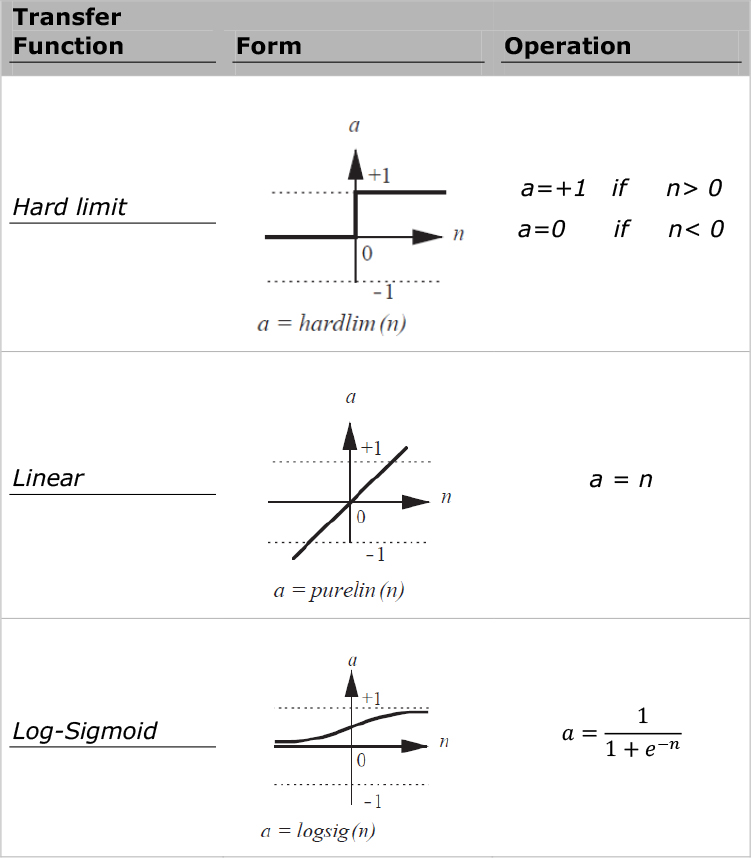
Just to provide an illustration, if in the previous example we had a hard limit transfer function, the actual output a would be a = hardlim(5) = 1. There are some guidelines for choosing the appropriate transfer function for each set of neurons in a network. These guidelines are especially robust for the neurons located at the output layer of the network. For example, if the nature of the output for a model is binary, we are advised to use Sigmoid transfer functions at the output layer so that it produces an output between 0 and 1, which represents the conditional probability of y = 1 given x or P(y = 1 ∣ x). Many neural network textbooks provide and elaborate on those guidelines at different layers in a neural network with some consistency and much disagreement, suggesting that the best practices should (and usually does) come from experience.
Typically, a neuron has more than a single input. In that case, each individual input pi can be shown as an element of the input vector p. Each of the individual input values would have its own adjustable weight wi of the weight vector W. Figure 9.4 shows a multiple-input neuron with R individual inputs.
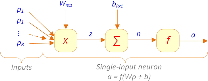
Figure 9.4 Typical Multiple-Input Neuron with R Individual Inputs
For this neuron, the net input n can be expressed as:
![]()
Considering the input vector p as a R × 1 vector and the weight vector W as a 1 × R vector, then n can be written in matrix form as:
![]()
where Wp is a scalar (i.e., 1 × 1 vector).
Moreover, each neural network is typically composed of multiple neurons connected to each other and structured in consecutive layers so that the outputs of a layer work as the inputs to the next layer. Figure 9.5 shows a typical neural network with three neurons at the input (i.e., first) layer, four neurons at the hidden (i.e., middle) layer, and a single neuron at the output (i.e., last) layer. Each of the neurons has its own weight, weighting function, bias, and transfer function and processes its own input(s) as described.
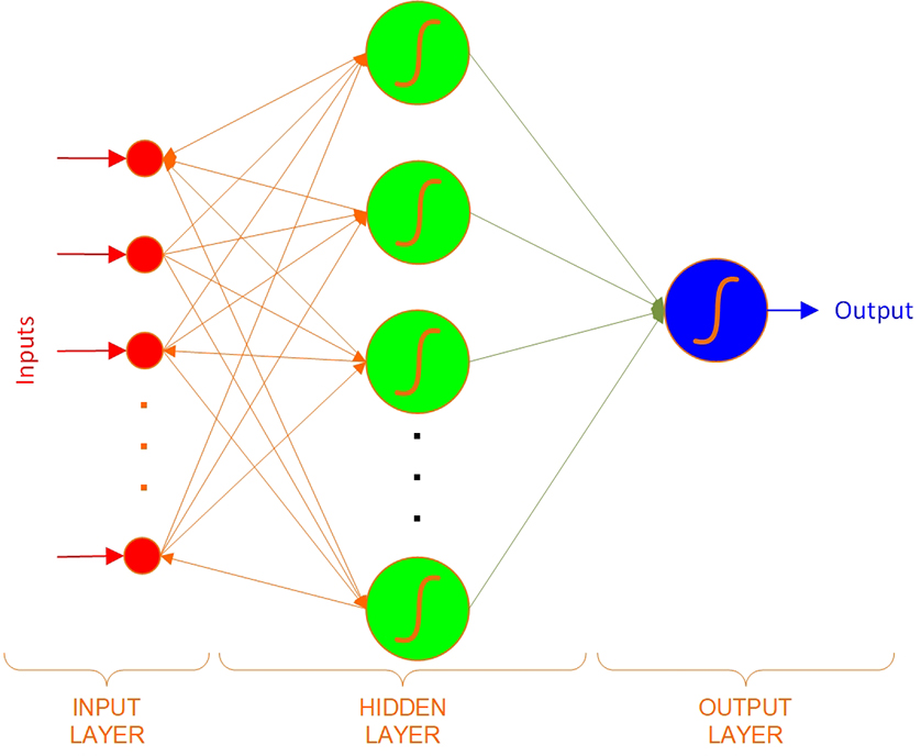
Figure 9.5 Typical Neural Network with Three Layers and Eight Neurons
While the inputs, weighting functions, and transfer functions in a given network are fixed, the values of the weights and biases are adjustable. The process of adjusting weights and biases in a neural network is what is commonly called training. In fact, in practice, a neural network cannot be used effectively for a prediction problem unless it is well trained by a sufficient number of examples with known actual outputs (a.k.a. targets). The goal of the training process is to adjust network weights and biases such that the network output for each set of inputs (i.e., each sample) is adequately close to its corresponding target value.
Elements of an Artificial Neural Network
A neural network is composed of processing elements that are organized in different ways to form the network’s structure. The basic processing unit in a neural network is the neuron. A number of neurons are then organized to establish a network of neurons. Neurons can be organized in a number of different ways; these various network patterns are referred to as topologies or network architecture. One of the most popular approaches, known as the feedforward-multi-layered perceptron, allows all neurons to link the output in one layer to the input of the next layer, but it does not allow any feedback linkage (Haykin, 2009).
Processing Element (PE)
The PE of an ANN is an artificial neuron. Each neuron receives inputs, processes them, and delivers a single output as shown in Figure 9.5. The input can be raw input data or the output of other processing elements. The output can be the final result (e.g., 1 means yes, 0 means no), or it can be input to other neurons.
Network Structure
Each ANN is composed of a collection of neurons that are grouped into layers. A typical structure is shown in Figure 9.6. Note the three layers: input, intermediate (called the hidden layer), and output. A hidden layer is a layer of neurons that takes input from the previous layer and converts those inputs into outputs for further processing. Several hidden layers can be placed between the input and output layers, although it is common to use only one hidden layer. In that case, the hidden layer simply converts inputs into a nonlinear combination and passes the transformed inputs to the output layer. The most common interpretation of the hidden layer is as a feature-extraction mechanism; that is, the hidden layer converts the original inputs in the problem into a higher-level combination of such inputs.
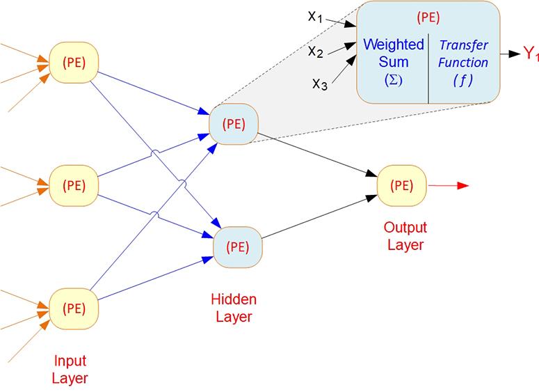
Figure 9.6 Neural Network with One Hidden Layer
PE: processing element (an artificial representation of a biological neuron); Xi: inputs to a PE; Y: output generated by a PE; Σ: summation function; and f: activation/transfer function.
In ANN, when information is processed, many of the processing elements perform their computations at the same time. This parallel processing resembles the way the human brain works, and it differs from the serial processing of conventional computing.
Input
Each input corresponds to a single attribute. For example, if the problem is to decide on approval or disapproval of a loan, attributes could include the applicant’s income level, age, and home ownership status. The numeric value, or the numeric representation of non-numeric value, of an attribute is the input to the network. Several types of data, such as text, picture, and voice, can be used as inputs. Preprocessing may be needed to convert the data into meaningful inputs from symbolic/non-numeric data or to numeric/scale data.
Outputs
The output of a network contains the solution to a problem. For example, in the case of a loan application, the output can be “yes” or “no.” The ANN assigns numeric values to the output, which may then need to be converted into categorical output using a threshold value so that the results would be 1 for “yes” and 0 for “no.”
Connection Weights
Connection weights are the key elements of an ANN. They express the relative strength (or mathematical value) of the input data or the many connections that transfer data from layer to layer. In other words, weights express the relative importance of each input to a processing element and, ultimately, to the output. Weights are crucial in that they store learned patterns of information. It is through repeated adjustments of weights that a network learns.
Summation Function
The summation function computes the weighted sums of all input elements entering each processing element. A summation function multiplies each input value by its weight and totals the values for a weighted sum. The formula for n inputs (represented with X) in one processing element is shown in Figure 9.7a, and for several processing elements, the summation function formulas are shown in Figure 9.7b.
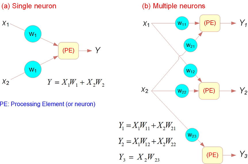
Figure 9.7 Summation Function for (a) a Single Neuron/PE and (b) Several Neurons/PEs
Transfer Function
The summation function computes the internal stimulation, or activation level, of the neuron. Based on this level, the neuron may or may not produce an output. The relationship between the internal activation level and the output can be linear or nonlinear. The relationship is expressed by one of several types of transformation (transfer) functions (see Table 9.1 for a list of commonly used activation functions). Selection of the specific activation function affects the network’s operation. Figure 9.8 shows the calculation for a simple sigmoid-type activation function example.
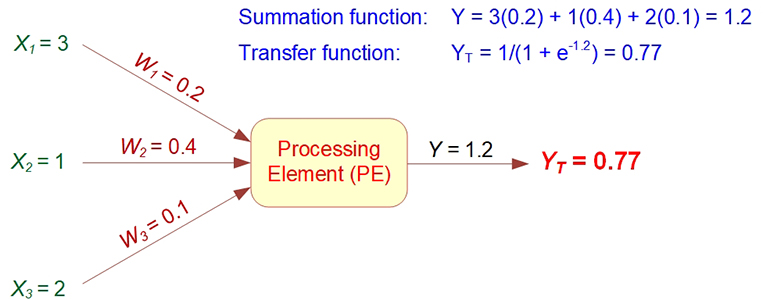
Figure 9.8 Example of ANN Transfer Function
The transformation modifies the output levels to fit within a reasonable range of values (typically between 0 and 1). This transformation is performed before the output reaches the next level. Without such a transformation, the value of the output becomes very large, especially when there are several layers of neurons. Sometimes a threshold value is used instead of a transformation function. A threshold value is a hurdle value for the output of a neuron to trigger the next level of neurons. If an output value is smaller than the threshold value, it will not be passed to the next level of neurons. For example, any value of 0.5 or less becomes 0, and any value above 0.5 becomes 1. A transformation can occur at the output of each processing element, or it can be performed only at the final output nodes.
Learning Process in ANN
In supervised learning, the learning process is inductive; that is, connection weights are derived from existing cases. The usual process of learning involves three tasks (see Figure 9.9):
1. Compute temporary outputs.
2. Compare outputs with desired targets.
3. Adjust the weights and repeat the process.
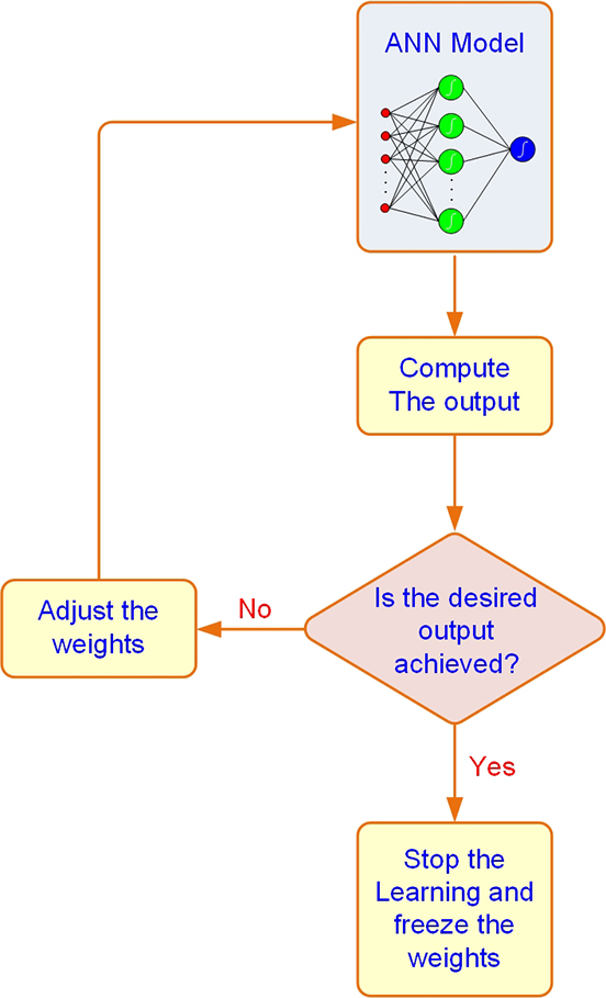
Figure 9.9 Supervised Learning Process of an ANN
Like any other supervised machine-learning technique, neural networks training is usually done by defining a performance function (F) (a.k.a. cost function or loss function) and optimizing (minimizing) that function by changing model parameters. Usually, the performance function is nothing but a measure of error (i.e., the difference between the actual input and the target) across all inputs of a network. There are several types of error measures (e.g., sum square errors, mean square errors, cross entropy, or even custom measures) when all of which are designed to capture the difference between the network outputs and the actual outputs.
The training process begins by calculating outputs for a given set of inputs using some random weights and biases. Once the network outputs are on hand, the performance function can be computed. The difference between the actual output (Y or YT) and the desired output (Z) for a given set of inputs is an error called delta (in calculus, the Greek symbol delta, Δ, means “difference”).
The objective is to minimize delta (i.e., reduce it to 0 if possible), which is done by adjusting the network’s weights. The key is to change the weights in the proper direction, making changes that reduce delta (i.e., error). Different ANNs compute delta in different ways, depending on the learning algorithm being used. Hundreds of learning algorithms are available for various situations and configurations of ANN.
Backpropagation for ANN Training
The optimization of performance (i.e., minimization of the error or delta) in the neural network is usually done by an algorithm called stochastic gradient descent (SGD), which is an iterative gradient-based optimizer used for finding the minimum (i.e., the lowest point) in performance functions, as in the case of neural networks. The idea behind the SGD algorithm is that the derivative of the performance function with respect to each current weight or bias indicates the amount of change in the error measure by each unit of change in that weight or bias element. These derivatives are referred to as network gradients. Calculation of network gradients in the neural networks requires application of an algorithm called backpropagation, which is the most popular neural network learning algorithm, that applies the chain rule of calculus to compute the derivatives of functions formed by composing other functions whose derivatives are known (more on the mathematical details of this algorithm can be found in Rumelhart, Hinton, and Williams (1986).
Backpropagation (short for back-error propagation) is the most widely used supervised learning algorithm in neural computing (Principe, Euliano, and Lefebvre, 2000). By using the SGD mentioned previously, the implementation of backpropagation algorithms is relatively straightforward. A neural network with backpropagation learning includes one or more hidden layers. This type of network is considered feedforward because there are no interconnections between the output of a processing element and the input of a node in the same layer or in a preceding layer. Externally provided correct patterns are compared with the neural network’s output during (supervised) training, and feedback is used to adjust the weights until the network has categorized all training patterns as correctly as possible (the error tolerance is set in advance).
Starting with the output layer, errors between network-generated actual output and the desired outputs are used to correct/adjust the weights for the connections between the neurons (see Figure 9.10). For any output neuron j, the error (delta) = (Zj - Yj) (df/dx) where Z and Y are the desired and actual outputs, respectively. Using the sigmoid function, f = [1 + exp(-x)]-1, where x is proportional to the sum of the weighted inputs to the neuron, is an effective way to compute the output of a neuron in practice. With this function, the derivative of the sigmoid function df/dx = f(1 - f) and of the error is a simple function of the desired and actual outputs. The factor f(1 - f) is the logistic function, which serves to keep the error correction well bounded. The weight of each input to the jth neuron is then changed in proportion to this calculated error. A more complicated expression can be derived to work backward in a similar way from the output neurons through the hidden layers to calculate the corrections to the associated weights of the inner neurons. This complicated method is an iterative approach to solving a nonlinear optimization problem that is very similar in meaning to the one characterizing multiple linear regression.
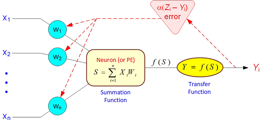
Figure 9.10 Backpropagation of Error for a Single Neuron
In backpropagation, the learning algorithm includes the following procedures:
1. Initialize weights with random values and set other parameters.
2. Read in the input vector and the desired output.
3. Compute the actual output via the calculations, working forward through the layers.
4. Compute the error.
5. Change the weights by working backward from the output layer through the hidden layers.
This procedure is repeated for the entire set of input vectors until the desired output and the actual output agree within some predetermined tolerance. Given the calculation requirements for one iteration, training a large network can take a very long time; therefore, in one variation, a set of cases is run forward and an aggregated error is fed backward to speed the learning. Sometimes, depending on the initial random weights and network parameters, the network does not converge to a satisfactory performance level. When this is the case, new random weights must be generated, and the network parameters, or even its structure, may have to be modified before another attempt is made. Current research is aimed at developing algorithms and using parallel computers to improve this process. For example, genetic algorithms (GA) can be used to guide the selection of the network parameters to maximize the performance of the desired output. In fact, most commercial ANN software tools are now using GA to help users “optimize” the network parameters in a semiautomated manner.
A central concern in the training of any type of machine-learning model is overfitting. It happens when the trained model is highly fitted to the training data set but performs poorly with regard to external data sets. Overfitting causes serious issues with respect to the generalizability of the model. A large group of strategies known as regularization strategies is designed to prevent models from overfitting by making changes or defining constraints for the model parameters or the performance function.
In the classic ANN models of small size, a common regularization strategy to avoid overfitting is to assess the performance function for a separate validation data set as well as the training data set after each iteration. Whenever the performance stopped improving for the validation data, the training process would be stopped. Figure 9.11 shows a typical graph of the error measure by the number of iterations of training. As shown, in the beginning, the error decreases in both training and validation data by running more and more iterations; but from a specific point (shown by the dashed line), the error starts increasing in the validation set while still decreasing in the training set. It means that beyond that number of iterations, the model becomes overfitted to the data set with which it is trained and cannot necessarily perform well when it is fed with some external data. That point actually represents the recommended number of iterations for training a given neural network.
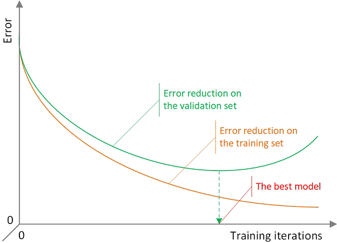
Figure 9.11 Illustration of the Overfitting in ANN—Gradually Changing Error Rates in the Training and Validation Data Sets As the Number of Iterations Increases
Deep Neural Networks
Until recently (before the advent of deep learning phenomenon), most neural network applications involved network architectures with only a few hidden layers and a limited number of neurons in each layer. Even in relatively complex business applications of neural networks, the number of neurons in networks hardly exceeded a few thousands. In fact, the processing capability of computers at the time was such a limiting factor that central processing units (CPU) were hardly able to run networks involving more than a couple of layers in a reasonable time. In recent years, development of graphics processing units (GPUs) along with the associated programming languages (e.g., CUDA by NVIDIA) that enable people to use them for data analysis purposes have led to more advanced applications of neural networks. GPU technology has enabled us to successfully run neural networks with over a million neurons. These larger networks are able to go deeper into the data features and extract more sophisticated patterns that could not be detected otherwise.
While deep networks can handle a considerably larger number of input variables, they also need relatively larger data sets to be trained satisfactorily; using small data sets for training deep networks typically leads to overfitting of the model to the training data and poor and unreliable results in case of applying to external data. Thanks to the Internet- and Internet of Things (IoT)-based data-capturing tools and technologies, larger data sets are now available in many application domains for deeper neural network training.
The input to a regular ANN model is typically an array of size R × 1, where R is the number of input variables. In the deep networks, however, we are able to use tensors (i.e., N-dimensional arrays) as input. For example, in image recognition networks, each input (i.e., image) can be represented by a matrix indicating the color codes used in the image pixels; or for video processing purposes, each video can be represented by several matrices (i.e., a 3D tensor), each representing an image involved in the video. In other words, tensors provide us with the ability to include additional dimensions (e.g., time, location) in analyzing the data sets.
Except for these general differences, the different types of deep networks involve various modifications to the architecture of standard neural networks that equip them with distinct capabilities of dealing with particular data types for advanced purposes. In the following section, we discuss some of these special network types and their characteristics.
Feedforward Multilayer Perceptron (MLP) Type Deep Networks
MLP deep networks, also known as deep feedforward networks, are the most general type of deep networks. These networks are simply large-scale neural networks that can contain many layers of neurons and handle tensors as their input. The types and characteristics of the network elements (i.e., weight functions, transfer functions) are pretty much the same as in the standard ANN models. These models are called feedforward because the flow of information that goes through them is always forwarding and no feedback connections (i.e., connections in which outputs of a model are fed back to itself) are allowed. The neural networks in which feedback connections are allowed are called recurrent neural networks (RNN). General RNN architectures as well as a specific variation of RNNs called long short-term memory networks are discussed in the later parts of this chapter.
Generally, a sequential order of layers has to be held between the input and the output layers in the MLP-type network architecture. This means that the input vector has to pass through all layers sequentially and cannot skip any of them; moreover, it cannot be directly connected to any layer except for the very first one; the output of each layer is the input to the subsequent layer. Figure 9.12 demonstrates a vector representation of the first three layers of a typical MLP network. As shown, there is only one vector going into each layer, which is either the original input vector (p for the first layer) or the output vector from the previous hidden layer in the network architecture (ai-1 for the ith layer). There are, however, some special variations of MLP network architectures designed for specialized purposes in which these principles can be violated.
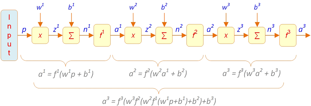
Figure 9.12 Vector Representation of the First Three Layers in a Typical MLP Network
Impact of Random Weights in Deep MLP
Optimization of the performance (loss) function in many real applications of deep MLPs is a challenging issue. The problem is that applying the common gradient-based training algorithms with random initialization of weights and biases that is very efficient for finding the optimal set of parameters in shallow neural networks most of the times could lead to getting stuck in the locally optimal solutions rather than catching the global optimum values for the parameters. As the depth of network increases, chances of reaching a global optimum using random initializations with the gradient-based algorithms decrease. In such cases, usually pretraining the network parameters using some unsupervised deep learning methods such as deep belief networks (DBNs) can be helpful (Hinton, Osindero, and Teh, 2006). DBNs are a type of a large class of deep neural networks called generative models. Introduction of DBNs in 2006 is considered as the beginning of the current deep learning renaissance (Goodfellow et al., 2016) since prior to that, deep models were considered too difficult to optimize. In fact, the primary application of DBNs today is to improve classification models by pretraining of their parameters.
Using these unsupervised learning methods, we can train the MLP layers, one at a time, starting from the first layer and use the output of each layer as the input to the subsequent layer and initialize that layer with an unsupervised learning algorithm. At the end, we will have a set of initialized values for the parameters across the whole network. Those pretrained parameters instead of random initialized parameters then can be used as the initial values in the supervised learning of the MLP. This pretraining procedure has been shown to cause significant improvements to the deep classification applications. Figure 9.13 illustrates the classification errors that resulted from training a deep MLP network with (blue circles) and without (black triangles) pretraining of parameters (Bengio, 2009). In this example, the blue line represents the observed error rates of testing a classification model (on 1,000 heldout examples) trained using a purely supervised approach with 10 million examples, whereas the black line indicates the error rates on the same testing data set when 2.5 million examples were initially used for unsupervised training of network parameters (using DBN) and then the other 7.5 million examples along with the initialized parameters were used to train a supervised classification model. The diagrams clearly show a significant improvement in terms of the classification error rate in the model pretrained by a deep belief network.
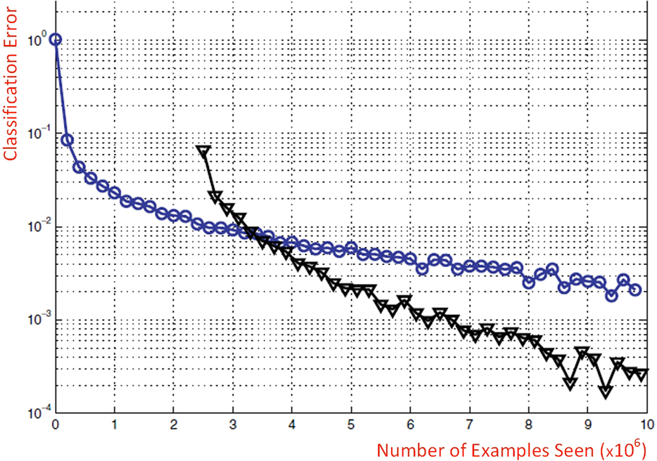
Figure 9.13 The Effect of Pretraining Network Parameters on Improving Results of a Classification Type Deep Neural Network
More Hidden Layers Versus More Neurons?
An important question regarding the deep MLP models is “Would it make sense (and produce better results) to restructure such networks with only a few layers, but many neurons in each?” In other words, the question is why do we need deep MLP networks with many layers when we can include the same number of neurons in just a few layers (i.e., wide networks instead of deep networks). According to the universal approximation theorem (Cybenko, 1989; Hornik, 1991), a sufficiently large single-layer MLP network will be able to approximate any function. Although theoretically founded, such a layer with many neurons may be prohibitively large and hence may fail to learn the underlying patterns correctly. A deeper network can reduce the number of neurons required at each layer and hence decrease the generalization error. Whereas theoretically it is still an open research question, practically using more layers in a network seems to be more effective and computationally more efficient than using many neurons in a few layers.
Like typical artificial neural networks, multilayer perceptron networks can also be used for various prediction, classification, and clustering purposes. Especially when a large number of input variables are involved or in cases that the nature of input has to be an N-dimensional array, a deep multilayer network design needs to be employed.
Convolutional Neural Networks
CNNs (LeCun et al., 1989) are among the most popular types of deep learning methods. CNNs are in essence variations of the deep MLP architecture, initially designed for computer vision applications (e.g., image processing, video processing, text recognition) but are also applicable to non-image data sets.
The main characteristic of the convolutional networks is having at least one layer involving a convolution weight function instead of general matrix multiplication. Figure 9.14 illustrates a typical convolutional unit.
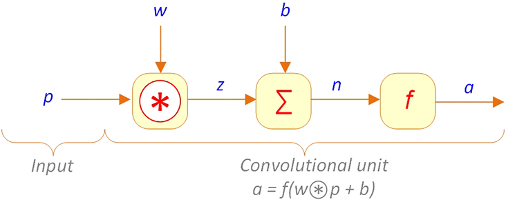
Figure 9.14. Typical Convolutional Network Unit
Convolution, typically shown by the symbol, is a linear operation that essentially aims at extracting simple patterns from sophisticated data patterns. For instance, in processing an image containing several objects and colors, convolution functions can extract simple patterns like the existence of horizontal or vertical lines or edges in different parts of the picture. We discuss convolution functions in more detail in the next section.
A layer containing a convolution function in a CNN is called a convolution layer. This layer is often followed by a pooling (a.k.a. subsampling) layer. Pooling layers are in charge of consolidating the large tensors to one with a smaller size and reduce the number of model parameters while keeping their important features. Different types of pooling layers are also discussed in the following sections.
Convolution Function
In the description of MLP networks, it was said that the weight function is generally a matrix manipulation function that multiplies the weight vector into the input vector to produce the output vector in each layer. Having a very large input vector/tensor, which is the case in most deep learning applications, we need a large number of weight parameters so that each single input to each neuron could be assigned a single weight parameter. For instance, in an image-processing task using a neural network for images of size 150 × 150 pixels, each input matrix will contain 22,500 (i.e., 150 times 150) integers, each of which should be assigned its own weight parameter per each neuron it goes into throughout the network. Therefore, having even only a single layer requires thousands of weight parameters to be defined and trained. As one might guess, this fact would dramatically increase the required time and processing power to train a network since in each training iteration, all of those weight parameters have to be updated by the SGD algorithm. The solution to this problem is the convolution function.
The convolution function can be thought of as a trick to address the issue defined in the previous paragraph. The trick is called parameter sharing, which in addition to computational efficiency provides additional benefits. Specifically, in a convolution layer, instead of having a weight for each input, there is a set of weights referred to as the convolution kernel or filter, which is shared between inputs and moves around the input matrix to produce the outputs.
Pooling
Most of the times, a convolution layer is followed by another layer known as the pooling (a.k.a. subsampling) layer. The purpose of a pooling layer is to consolidate elements in the input matrix to produce a smaller output matrix while maintaining the important features. Normally, a pooling function involves an r × c consolidation window (similar to a kernel in the convolution function) that moves around the input matrix and in each move calculates some summary statistics of the elements involved in the consolidation window so that it can be put it in the output image. For example, a particular type of pooling functions called average pooling takes the average of the input matrix elements involved in the consolidation window and puts that average value as an element of the output matrix in the corresponding location. Similarly, the max pooling function (Zhou et al., 1988) takes the maximum of the values in the window as the output element. Unlike convolution, for the pooling function, given the size of the consolidation window (i.e., r and c), stride should be carefully selected so that there would be no overlaps in the consolidations. The pooling operation using an r × c consolidation window reduces the number of rows and columns of the input matrix by a factor of r and c, respectively. For example, using a 3 × 3 consolidation window, a 15 × 15 matrix will be consolidated to a 5 × 5 matrix.
Pooling, in addition to reducing the number of parameters, is especially useful in the image-processing applications of deep learning in which the critical task is to determine whether a feature (e.g., a particular animal) is present in an image while the exact spatial location of the same in the picture is not important. However, if the location of features is important in a particular context, applying a pooling function could potentially be misleading.
There are various types of pooling operations such as max pooling, average pooling, the L2 norm of a rectangular neighborhood, and weighted average pooling. The choice of proper pooling operation as well as the decision to include a pooling layer in the network depends highly on the context and properties of the problem that the network is solving.
Image Processing Using Convolutional Networks
Real applications of deep learning in general and CNNs in particular highly depend on the availability of large, annotated data sets. Theoretically, CNNs can be applied to many practical problems, and today there are many large and feature-rich databases for such applications available. Nevertheless, the biggest challenge is that in supervised learning applications, one needs an already annotated (i.e., labeled) data set to train the model before we can use it for prediction/identification of other unknown cases. Whereas extracting features of data sets using CNN layers is an unsupervised task, the extracted features will not be much use without having labeled cases to develop a classification network in a supervised learning fashion. That is why image classification networks traditionally involve two pipelines: visual feature extraction and image classification.
ImageNet (http://www.image-net.org) is an ongoing research project that provides researchers with a large database of images each linked to a set of synonym words (known as synset) from WordNet (a word hierarchy database). Each sysnet represents a particular concept in the WordNet. Currently, WordNet includes more than 100,000 synsets, each of which is supposed to be illustrated by an average of 1,000 images in the ImageNet. ImageNet is a huge database for developing image-processing-type deep networks. It contains more than 15 million labeled images in 22,000 categories. Because of its sheer size and proper categorization, ImageNet is by far the most widely used benchmarking data set to assess the efficiency and accuracy of deep networks designed by deep learning researchers.
One of the first convolutional networks designed for image classification using the ImageNet data set was AlexNet (Krizhevsky, Sutskever, and Hinton, 2012). It was composed of five convolution layers followed by three fully connected (a.k.a. dense) layers (see Figure 9.15 for a schematic representation of AlexNet). One of the contributions of this relatively simple architecture that made its training remarkably faster and computationally efficient was the use of rectified linear unit (ReLu) transfer functions in the convolution layers instead of the traditional sigmoid functions. By doing so, the designers addressed the issue called the vanishing gradient problem caused by very small derivatives of sigmoid functions in some regions of the images. The other important contribution of this network that has a dramatic role in improving the efficiency of deep networks was the introduction of the concept of dropout layers to the CNNs as a regularization technique to reduce overfitting. A dropout layer typically comes after the fully connected layers and applies a random probability to the neurons to switch off some of them and make the network sparser.
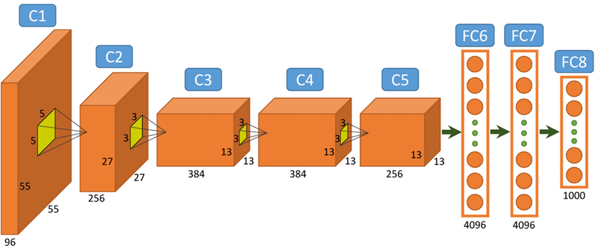
Figure 9.15 Architecture of AlexNet, a Convolutional Network for Image Classification
In the recent years, in addition to a large number of data scientists who showcase their deep learning capabilities, a number of well-known industry-leading companies such as Microsoft, Google, and Facebook have participated in the annual ImageNet Large Scale Visual Recognition Challenge (ILSVRC). The goal in the ILSVRC classification task is to design and train networks that are capable of classifying 1.2 million input images into one of the 1,000 image categories. For instance, GoogLeNet (a.k.a. Inception), a deep convolutional network architecture designed by Google researchers, was the winning architecture of ILSVRC 2014 with a 22-layer network and only a 6.66 percent classification error rate, only slightly (5.1%) worse than the human-level classification error (Russakovsky et al., 2015). The main contribution of the GoogLeNet architecture was to introduce a module called Inception. The idea of Inception is that because one would have no idea about what size of convolution kernel would perform the best on a particular data set, it is better to include multiple convolutions and let the network decide which one to use. Therefore, as shown in Figure 9.16, in each convolution layer, the data coming from the previous layer is passed through multiple types of convolution and the outputs are concatenated before going to the next layer. Such architecture allows the model to take into account both local features via smaller convolutions and high abstracted features via larger ones.
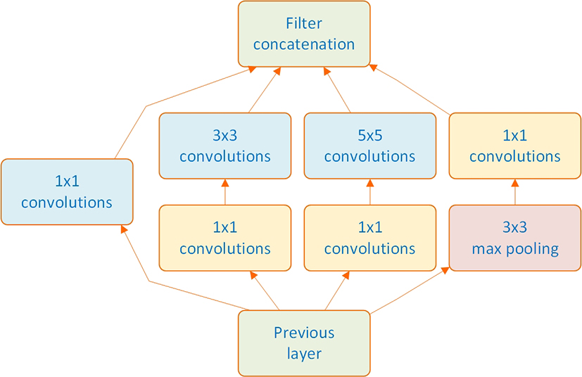
Figure 9.16 Conceptual Representation of the Inception Feature in GoogLeNet
Google recently launched a new service, Google Lens, that uses deep learning artificial neural network algorithms (along with other AI techniques) to deliver information about the images captured by users from their nearby objects. This involves identifying the objects, products, plants, animals, and locations and providing information about them on the Internet. Some other features of this service are the capability of saving contact information from a business card image on the phone, identifying type of plants and breed of animals, identifying books and movies from their cover photos, and providing information (e.g., stores, theaters, shopping, reservations) about them. Figure 9.17 shows two examples of using the Google Lens app on an Android mobile device.

Figure 9.17 Two Examples of Using the Google Lens, a Service Based on Convolutional Deep Networks for Image Recognition.
Even though later on more accurate networks have been developed (e.g., He et al, 2015) in terms of efficiency and processing requirements (i.e., smaller number of layers and parameters), GoogLeNet is considered to be one of the best architectures to date. Apart from AlexNet and GoogLeNet, several other convolutional network architectures such as Residual Networks (ResNet), VGGNet, and Xception have been developed and contributed to the image-processing area, all relying on the ImageNet database.
In a May 2018 effort to address the labor-intensive task of labeling images on a large scale, Facebook published a weakly supervised training image recognition deep learning project (Mahajan et al., 2018). This project used hashtags made by the users on the images posted on Instagram as labels and trained a deep learning image recognition model based on that. The model was trained using 3.5 billion Instagram images labeled with around 17,000 hashtags using 336 GPUs working in parallel; the training procedure took a few weeks to be accomplished. A preliminary version of the model (trained using only 1 billion images and 1,500 hashtags) was then tested on the ImageNet benchmark data set and is reported to have outperformed the state-of-the-art models in terms of accuracy by more than 2 percent. This big achievement by Facebook surely will open doors to a new world of image processing using deep learning since it can dramatically increase the size of available image data sets that are labeled for training purposes.
Text Processing Using Convolutional Networks
In addition to image processing, which was in fact the main reason for the popularity and development of convolutional networks, they have been shown to be useful in some large-scale text mining tasks as well. Especially since 2013, when Google published its word2vec project (Mikolov et al., 2013a, 2013b), the applications of deep learning for text mining have increased remarkably.
Word2vec is a two-layer neural network that gets a large text corpus as the input and converts each word in the corpus to a numeric vector of any given size (typically ranging from 100 to 1,000) with very interesting features. Although word2vec itself is not a deep learning algorithm, its outputs (word vectors also known as word embeddings) already have been widely used in many deep learning research and commercial projects as inputs.
One of the most interesting properties of word vectors created by the word2vec algorithm is maintaining the words’ relative associations. For example, vector operations
<DM>vector('King')−vector('Man')+vector('Woman')</DM>
and
<DM>vector('London')−vector('England')+vector('France')</DM>
will result in a vector very close to vector(‘Queen’) and vector(‘Paris’), respectively. Figure 9.18 shows a simple vector representation of the first example in a two-dimensional vector space.
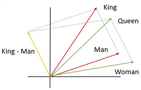
Figure 9.18. Typical Vector Representation of Word Embeddings in a Two-Dimensional Space
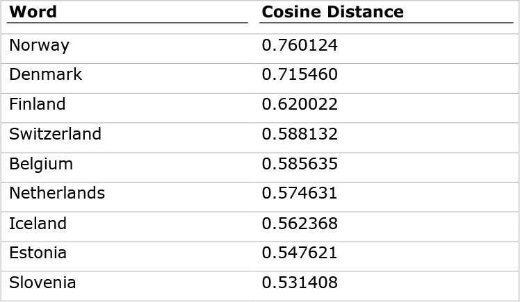
Moreover, the vectors are specified in such a way that those of a similar context are placed very close to each other in the n-dimensional vector space. For instance, in the word2vec model pretrained by Google using a corpus including about 100 billion words (taken from Google News), the closest vectors to the vector (‘Sweden’) in terms of cosine distance, as shown in Table 9.2, identifies European country names near the Scandinavian region, the same region in which Sweden is located.
Table 9.2. Example of the word2vec Project Indicating the Closest Word Vectors to the Word “Sweden”
Additionally, since word2vec takes into account the contexts in which a word has been used and the frequency of using it in each context in guessing the meaning of the word, enabling us to represent each term with its semantic context instead of just the syntactic/symbolic term itself. As a result, word2vec addresses several word variation issues that used to be problematic in traditional text mining activities. In other words, word2vec is able to handle and correctly represent words including typos, abbreviations, and informal conversations. For instance, the words Frnce, Franse, and Frans would all get roughly the same word embeddings as their original counterpart France. Word embeddings are also able to determine other interesting types of associations such as distinction of entities (e.g., vector[‘human’]-vector[‘animal’]~vector[‘ethics’]) or geopolitical associations (e.g., vector[‘Iraq’] – vector[‘violence’]~ vector[‘Jordan’]).
By providing such a meaningful representation of textual data, in recent years, the word2vec has driven many deep learning–based text mining projects in a wide range of contexts (e.g., medical, computer science, social media, marketing), and various types of deep networks have been applied to the word embeddings created by this algorithm to accomplish different objectives.
Recurrent Networks and Long Short-Term Memory Networks
Human thinking and understanding to a great extent rely on context. It is crucial for us, for example, to know that a particular speaker uses very sarcastic language (based on his previous speeches) to fully catch all the jokes that he makes. Or to understand the real meaning of the word fall (i.e., either the season or to collapse) in the sentence “It is a nice day of fall.”, without knowledge about the other words in the surrounding sentences, would only be guessing not necessarily understanding. Knowledge of context is typically formed based on observing events that happened in the past. In fact, human thoughts are persistent, and we use every piece of information we previously acquired about an event in the process of analyzing it rather than throwing away our past knowledge and thinking from scratch every time we face similar events or situations. Hence, there seems to be a recurrence in the way humans process information.
While deep MLP and convolutional networks are specialized for processing a static grid of values like an image or a matrix of word embeddings, sometimes the sequence of input values is also important to the operation of the network to accomplish a given task and hence should be taken into account. Another popular type of neural networks is recurrent neural network (RNN) (Rumelhart et al., 1986) that is specifically designed to process sequential inputs. An RNN basically models a dynamic system where (at least in one of its hidden neurons) the state of the system (i.e., output of a hidden neuron) at each time point t depends on both the inputs to the system at that time as well as its state at the previous time point t-1. In other words, RNNs are the type of neural networks that have memory and that apply that memory to determine their future outputs. For instance, in designing a neural network to play chess, it is important to take into account several previous moves while training the network,because a wrong move by a player can lead to the eventual loss of the game in the subsequent 10 to 15 plays. Also, to understand the real meaning of a sentence in an essay, sometimes we need to rely on the information portrayed in the previous several sentences or paragraphs. That is, for a true understanding, we need the context built sequentially and collectively over time. Therefore, it is crucial to consider a memory element for the neural network that takes into account the effect of prior moves (in the chess example) and prior sentences and paragraphs (in the essay example) to determine the best output. This memory portrays and creates the context required for the learning and understanding.
In static networks like MLP-type CNNs, we are trying to find some functions (i.e., network weights and biases) that map the inputs to some outputs that are as close as possible to the actual target. In dynamic networks like RNNs, on the other hand, both inputs and outputs are sequences (patterns). Therefore, a dynamic network is a dynamic system rather than a function because its output depends not only on the input but also on the previous outputs.
Graphically, a recurrent unit in a network can be depicted in a circuit diagram like the one shown in Figure 9.19. In this figure, D represents the tap delay lines, or simply the delay element of the network that, at each time point t, contains a(t), the previous output value of the unit. Sometimes instead of just one value, we store several previous output values in D to account for the effect of all of them. Also, iw and lw represent the weight vectors applied to the input and the delay, respectively.
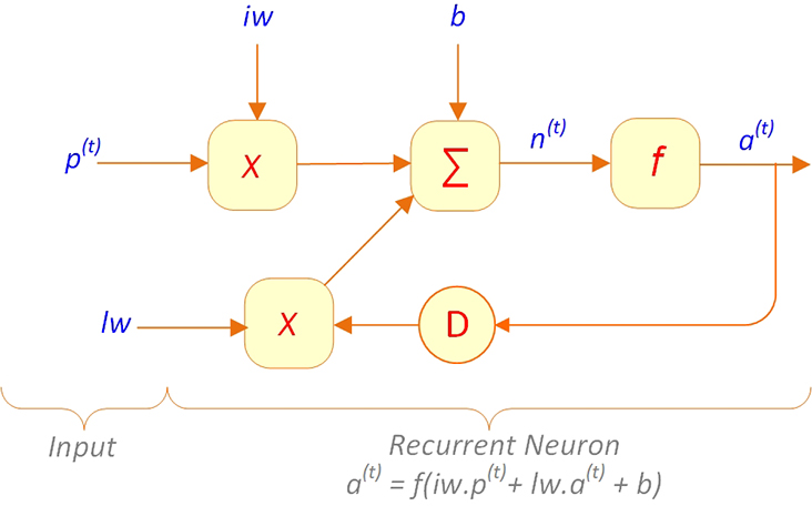
Figure 9.19 Typical Recurrent Unit
Technically speaking, any network with feedback can actually be called a deep network. Because even with a single layer, the loop created by the feedback can be thought of as a static MLP-type network with many layers (see Figure 9.20 for a graphical illustration of this structure). However, in practice, each recurrent neural network would involve dozens of layers, each with feedback to itself, or even to the previous layers, which makes a recurrent neural network even deeper and more complicated.
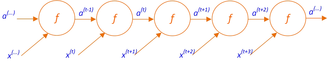
Figure 9.20 Unfolded View of a Typical Recurrent Network
Because of the feedbacks, computation of gradients in the recurrent neural networks would be somewhat different from the general backpropagation algorithm used for the static MLP networks. There are two alternative approaches for computing the gradients in the RNNs, namely, real-time recurrent learning (RTRL) and backpropagation through time (BTT), whose explanation is beyond the scope of this chapter. Nevertheless, the general purpose remains the same; once the gradients have been computed, the same procedures are applied to optimize the learning of the network parameters.
Long-Short Term Memory Networks
The long short-term memory (LSTM) networks (Hochreiter & Schmidhuber, 1997) are variations of recurrent neural networks that today are known as the most effective sequence modeling technique and are the base of many practical applications. In a dynamic network, the weights are called the long-term memory while the feedbacks role is the short-term memory.
In essence, only the short-term memory (i.e., feedbacks; previous events) provides a network with the context. In a typical RNN, the information on the short-term memory is continuously replaced as new information is fed back into the network over time. That is why RNNs perform well when the gap between the relevant information and the place that is needed is small. For instance, for predicting the last word in the sentence “The referee blew his whistle,” we just need to know a few words back (i.e., the referee) to correctly predict. Since in this case the gap between the relevant information (i.e., the referee) and where it is needed (i.e., to predict whistle) is small, an RNN network can easily perform this learning and prediction task.
However, sometimes the relevant information required to perform a task is far away from where it is needed (i.e., the gap is large). Therefore, it is quite likely that it would have already been replaced by other information in the short-term memory by the time it is needed for the creation of the proper context. For instance, to predict the last word in “I went to a carwash yesterday. It cost $5 to wash my car,” there is a relatively larger gap between the relevant information (i.e., carwash) and where it is needed. Sometimes we may even need to refer to the previous paragraphs to reach the relevant information for predicting the true meaning of a word. In such cases, RNNs usually do not perform well since they cannot keep the information in their short-term memory for a long enough time. Fortunately, LSTM networks do not have such a shortcoming. The term long short-term memory network then refers to a network in which we are trying to remember what happened in the past (i.e., feedbacks; previous outputs of the layers) for a long enough time so that it can be used/leveraged in accomplishing the task when needed.
From an architectural viewpoint, the memory concept (i.e., remembering “what happened in the past”) is incorporated in LSTM networks by incorporating four additional layers into the typical recurrent network architecture; three gate layers, namely input gate, forget (a.k.a. feedback) gate, and output gate, and an additional layer called Constant Error Carousel (CEC), also known as the state unit that integrates those gates and interacts them with the other layers. Each gate is nothing but a layer with two inputs, one from the network inputs and the other a feedback from the final output of the whole network. The gates involve log-sigmoid transfer functions. Therefore, their outputs will be between 0 and 1 and describe how much of each component (either input, feedback, or output) should be let through the network. Also, CEC is a layer that falls between the input and the output layers in a recurrent network architecture and applies the gates outputs to make the short-term memory long.
To have a long short-term memory means that we want to keep the effect of previous outputs for a longer time. However, we typically do not want to indiscriminately remember everything that has happened in the past. Therefore, gating provides us with the capability of remembering prior outputs selectively. The input gate will allow selective inputs to the CEC; the forget gate will clear the CEC from the unwanted previous feedbacks; and the output gate will allow selective outputs from the CEC. Figure 9.21 shows a simple depiction of a typical LSTM architecture.
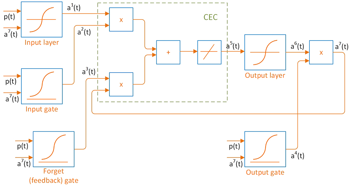
Figure 9.21 Typical Long Short-Term Memory (LSTM) Network Architecture
In summary, the gates in the LSTM are in charge of controlling the flow of information through the network and dynamically change the time scale of integration based on the input sequence. As a result, LSTM networks are able to learn long-term dependencies among the sequence of inputs more easily than the regular RNNs.
LSTM Networks Applications
Since their emergence in the late 1990s (Hochreiter & Schmidhuber, 1997), LSTM networks have been widely used in many sequence modeling applications including image captioning (i.e., automatically describing the content of images) (Vinyals et al., 2017, 2015), handwriting recognition and generation (Graves, 2013; Keysers et al., 2017), parsing (Liang et al., 2016), speech recognition (Graves and Jaitly, 2014), and machine translation (Bahdanau et al., 2014; Sutskever et al., 2014).
Currently, we are surrounded by multiple deep learning solutions working on the basis of speech recognition, such as Apple’s Siri, Google Now, Microsoft’s Cortana, and Amazon’s Alexa, several of which we deal on a daily basis (e.g., checking on the weather, asking for a Web search, calling a friend, and asking for directions on the map). Note taking is not a difficult, frustrating task anymore since we can easily record a speech or lecture, upload the digital recording on one of the several cloud-based speech-to-text service providers’ platforms and download the transcript in a few seconds. The Google cloud-based speech-to-text service, for example, supports 120 languages and their variants and has the ability to convert speech to text either in real time or using recorded audios. The Google service automatically handles the noise in the audio; accurately punctuates the transcripts with commas, question marks, and periods; and can be customized by the user to a specific context by getting a set a terms and phrases that are very likely to be used in a speech and recognizing them appropriately.
In 2014, Microsoft launched its Skype Translator service, a free voice translation service involving both speech recognition and machine translation with the ability of translating real-time conversations in 10 languages. Using this service, people with different languages can talk to each other in their own languages via a Skype voice or video call, and the system recognizes their voices and translates their every sentence spoken by a translator bot in near real time for the other party. To provide more accurate translations, the deep networks used in the backend of this system were trained using conversational language (i.e., using materials such as translated Web pages, movie subtitles, and casual phrases taken from people’s conversations in social networking Web sites) rather than the formal language commonly used in documents. The output of the speech recognition module of the system then goes through TrueText, a Microsoft technology for normalizing text that is capable of identifying mistakes and disfluencies (e.g., pauses during the speech or repeating some parts of speech, or adding fillers like “um” and “ah” when speaking) that people commonly conduct in their conversations and account for them for making better translations. Figure 9.22 shows the four-step process involved in the Skype Translator by Microsoft, each of which relies on the LSTM type of deep neural networks.
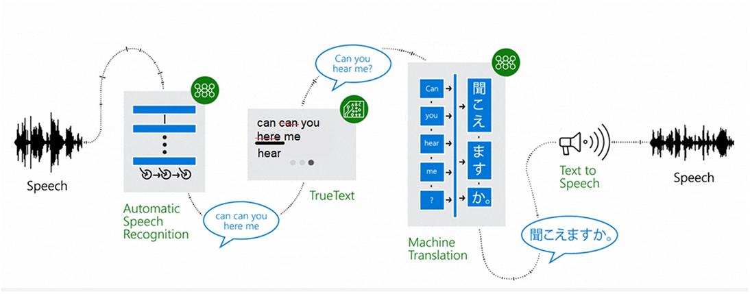
Figure 9.22 Four-Step Process of Translating Speech Using Deep Networks in the Microsoft Skype Translator
Computer Frameworks for Implementation of Deep Learning
Advances in deep learning owe its recent popularity, to a great extent, to advances in the software and hardware infrastructure required for its implementation. In the past few decades, GPUs have been revolutionized to support the playing of high-resolution videos as well as advanced video games and virtual reality applications. However, GPUs’ huge processing potential had not been effectively utilized for purposes other than graphics processing up until a few years ago. Thanks software libraries such as Theano (Bergstra et al., 2010), Torch (Collobert, Kavukcuoglu, and Farabet, 2011), Caffe (Jia et al., 2014), PyLearn2 (Goodfellow et al., 2013), Tensorflow (Abadi et al., 2016), and MXNet (Chen et al., 2015) developed with the purpose of programming GPUs for general-purpose processing (just as CPUs), and particularly for deep learning and analysis of Big Data GPUs have become a critical enabler for the modern day analytics. The operation of these libraries mostly relies on a parallel computing platform and application programming interface (API) developed by NVIDIA called Compute Unified Device Architecture (CUDA), which enables software developers to use GPUs made by NVIDIA for general-purpose processing. In fact, each deep learning framework consists of a high-level scripting language (e.g., Python, R, Lua) and a library of deep learning routines usually written in C (for using CPUs) or CUDA (for using GPUs).
We next introduce some of the most popular software libraries used for deep learning by researchers and practitioners, including Torch, Caffe, Tensorflow, Theano, and Keras, and discuss some of their specific properties.
Torch
Torch (Collobert et al., 2011) is an open source scientific computing framework (available at www.torch.ch) for implementing machine-learning algorithms using GPUs. The Torch framework is a library based on LuaJIT, a compiled version of the popular Lua programming language (www.lua.org). In fact, Torch adds a number of valuable features to Lua that make deep learning analyses possible; Torch enables supporting N-dimensional arrays (i.e., tensors) whereas tables (i.e., 2-dimensional arrays) normally are the only data-structuring method used by Lua. Additionally, Torch includes routine libraries for manipulating (i.e., indexing, slicing, transposing) tensors, linear algebra, neural network functions, and optimization. More importantly, while Lua by default uses CPU to run the programs, Torch enables use of GPUs for running programs written in the Lua language.
The easy and extremely fast scripting properties of LuaJIT along with its flexibility have made Torch a very popular framework for practical deep learning applications such that today its latest version, Torch7, is widely used by a number of big companies in the deep learning area including Facebook, Google, and IBM in their research labs as well as for their commercial applications.
Caffe
Caffe is another open source deep learning framework (available at http://caffe.berkeleyvision.org) created by Yangqing Jia (2013), a PhD student at the University of California–Berkeley, which the Berkeley AI Research (BAIR then further developed). Caffe has multiple options to be used as a high-level scripting language including the command line, Python, and MATLAB interfaces. The deep learning libraries in Caffe are written in the C++ programming language.
In Caffe, everything is done using text files instead of code. That is, to implement a network, generally we need to prepare two text files with the .prototxt extension that are communicated by the Caffe engine via JavaScript Object Notation (JSON) format. The first text file, known as the architecture file, defines the architecture of the network layer by layer where each layer is defined by a name, a type (e.g., data, convolution, output), the names of its previous (bottom) and next (top) layers in the architecture, and some required parameters (e.g., kernel size and stride for a convolutional layer). The second text file, known as the solver file, specifies the properties of the training algorithm including the learning rate, maximum number of iterations, and processing unit (CPU or GPU) to be used for training the network.
While Caffe supports multiple types of deep network architectures like CNN and LSTM, it is particularly known to be an efficient framework for image processing due to its incredible speed in processing image files. According to its developers, it is able to process over 60 million images per day (i.e., 1 ms/image) using a single NVIDIA K40 GPU. In 2017, Facebook released an improved version of Caffe called Caffe2 (www.caffe2.ai) with the aim of improving the original framework to be effectively used for deep learning architectures other than CNN and with a special emphasis on portability for performing cloud and mobile computations while maintaining scalability and performance.
TensorFlow
Another popular open source deep learning framework is TensorFlow. It was originally developed and written in Python and C++ by the Google Brain Group in 2011 as DistBelief, but it was further developed into TensorFlow in 2015. TensorFlow at this time is the only deep learning framework that, in addition to CPUs and GPUs, supports Tensor Processing Units (TPUs), a type of processor developed by Google in 2016 for the specific purpose of neural network machine learning. In fact, TPUs were specifically designed by Google for the TensorFlow framework.
Although Google has not yet made TPUs available to the market, it is reported that it has used them in a number of its commercial services such as Google search, Street View, Google Photos, and Google Translate with significant improvements reported. A detailed study performed by Google shows that TPUs deliver 30 to 80 times higher performance per watt than contemporary CPUs and GPUs (Sato, Young, and Patterson, 2017). For example, it has been reported (Ung, 2016) that in Google Photos, an individual TPU can process over 100 million images per day (i.e., 0.86 ms/image). Such a unique feature will probably put TensorFlow way ahead of the other alternative frameworks in the near future as soon as Google makes TPUs commercially available.
Another interesting feature of TensorFlow is its visualization module, TensorBoard. Implementing a deep neural network is a complex and confusing task. TensorBoard refers to a Web application involving a handful of visualization tools to visualize network graphs and plot quantitative network metrics with the aim of helping users to better understand what is going on during training procedures and to debug possible issues.
Theano
In 2007, the Deep Learning Group at the University of Montreal developed the initial version of a Python library, Theano (http://deeplearning.net/software/theano), to define, optimize, and evaluate mathematical expressions involving multi-dimensional arrays (i.e., tensors) on CPU or GPU platforms. Theano was one of the first deep learning frameworks but later became a source of inspiration for the developers of TensorFlow. Theano and TensorFlow both pursue a similar procedure in the sense that in both, a typical network implementation involves two sections; in the first section, a computational graph is built by defining the network variables and operations to be done on them; and the second section runs that graph (in Theano by compiling the graph into a function and in TensorFlow by creating a session). In fact, what happens in these libraries is that the user defines the structure of the network by providing some simple and symbolic syntax understandable even for beginners in programming, and the library automatically generates appropriate codes in either C (for processing on CPU) or CUDA (for processing on GPU) to implement the defined network. Hence, users without any knowledge of programming in C or CUDA and with just a minimum knowledge of Python are able to efficiently design and implement deep learning networks on the GPU platforms.
Theano also includes some built-in functions to visualize computational graphs as well as to plot the network performance metrics even though its visualization features are not comparable to TensorBoard.
Keras: An Application Programming Interface
While all of the previously described deep learning frameworks require users to be familiar with their own syntax (through reading their documentations) to be able to successfully train a network, fortunately there are some easier, more user-friendly ways to do so. Keras (https://keras.io/) is an open source neural network library written in Python that functions as a high-level application programming interface (API) and is able to run on top of various deep learning frameworks including Theano and TensorFlow. In essence, Keras just by getting the key properties of network building blocks (i.e., type of layers, transfer functions, and optimizers) via an extremely simple syntax automatically generates syntax in one of the deep learning frameworks and runs that framework in the backend. While Keras is efficient enough to build and run general deep learning models in just a few minutes, it does not provide several advanced operations provided by TensorFlow or Theano. Therefore, in dealing with special deep network models that require advanced settings, one still needs to directly use those frameworks instead of Keras (or other APIs such as Lasagne) as a proxy.
Cognitive Computing
We are witnessing a significant increase in the way technology is evolving. Things that once took decades are now taking months, and the things that we see only in SciFi movies are becoming reality, one after another. Therefore, it is safe to say that in the next decade or two, technological advancements will transform how people live, learn, and work in a rather dramatic fashion. The interactions between humans and technology will become intuitive, seamless, and perhaps transparent. Cognitive computing will have a significant role to play in this transformation. Generally speaking, cognitive computing refers to the computing systems that use mathematical models to emulate (or partially simulate) the human cognition process to find solutions to complex problems and situations where the potential answers can be imprecise. While the term cognitive computing is often used interchangeably with AI and smart search engines, the phrase itself is closely associated with IBM’s cognitive computer system Watson and its success on the television show, Jeopardy! Details on Watson’s success on Jeopardy! can be found at the end of Chapter 1.
According to Cognitive Computing Consortium (2018), cognitive computing makes a new class of problems computable. It addresses highly complex situations that are characterized by ambiguity and uncertainty; in other words, it handles the kinds of problems that are thought to be solvable by human ingenuity and creativity. In today’s dynamic, information-rich, and unstable situations, data tend to change frequently, and they often conflict. The goals of users evolve as they learn more and redefine their objectives. To respond to the fluid nature of users’ understanding of their problems, the cognitive computing system offers a synthesis not just of information sources but also of influences, contexts, and insights. To achieve such a high-level of performance, cognitive systems often need to weigh conflicting evidence and suggest an answer that is “best” rather than “right.” Figure 9.23 illustrates a general framework for cognitive computing where data and AI technologies are used to solve complex real-world problem.
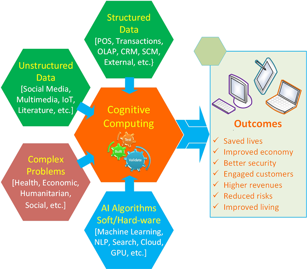
Figure 9.23 Conceptual Framework for Cognitive Computing and Its Promises
How Does Cognitive Computing Work?
As one would guess from the name, cognitive computing works much like a human thought process, reasoning mechanism, and cognitive system. These cutting-edge computation systems can find and synthesize data from various information sources and weigh context and conflicting evidence inherent in the data to provide the best possible answers to a given question or problem. To achieve this, cognitive systems include self-learning technologies that use data mining, pattern recognition, deep learning, and NLP to mimic the way the human brain works.
Using computer systems to solve the types of problems that humans are typically tasked with requires vast amounts of structured and unstructured data fed to machine-learning algorithms. Over time, cognitive systems are able to refine the way in which they learn and recognize patterns and the way they process data to become capable of anticipating new problems and modeling and proposing possible solutions.
To achieve those capabilities, cognitive computing systems must have the following key attributes as defined by the Cognitive Computing Consortium (2018):
• Adaptive: Cognitive systems must be flexible enough to learn as information changes and goals evolve. The systems must be able to digest dynamic data in real time and make adjustments as the data and environment change.
• Interactive: Human-computer interaction (HCI) is a critical component in cognitive systems. Users must be able to interact with cognitive machines and define their needs as those needs change. The technologies must also be able to interact with other processors, devices, and cloud platforms.
• Iterative and stated problem: Cognitive computing technologies can also identify problems by asking questions or pulling in additional data if a stated problem is vague or incomplete. The systems do this by maintaining information about similar situations that have previously occurred.
• Contextual: Understanding context is critical in thought processes, so cognitive systems must understand, identify, and mine contextual data, such as syntax, time, location, domain, requirements, and a specific user’s profile, tasks, or goals. Cognitive systems may draw on multiple sources of information, including structured and unstructured data and visual, auditory, or sensor data.
How Does Cognitive Computing Differ from AI?
Cognitive computing is often used interchangeably with AI, the umbrella term used for technologies that rely on data and scientific methods/computations to make (or help/support in making) decisions. But there are differences between the two terms, which can largely be found within their purposes and applications. AI technologies include—but are not limited to—machine learning, neural computing, NLP, and, most recently, deep learning. With AI systems, especially in machine-learning systems, data are fed into the algorithm for processing (an iterative and time-demanding process that is often called training) so that the systems “learn” variables and interrelationships among those variables so that it can produce predictions (or characterizations) about a given complex problem or situation. Applications based on AI and cognitive computing include intelligent assistants, such as Amazon’s Alexa, Google Home, and Apple’s Siri. A simple comparison between cognitive computing and AI is given in Table 9.3 (Reynolds and Feldman, 2014; CCC, 2018).
Table 9.3. Cognitive Computing Versus Artificial Intelligence (AI)
As can be seen in Table 9.3, the differences between AI and cognitive computing is rather marginal. This is expected because cognitive computing is often characterized as a subcomponent of AI or an application of AI technologies tailored for a specific purpose. AI and cognitive computing both utilize similar technologies and are applied to similar industry segments and verticals. The main difference between the two is the purpose: while cognitive computing is aimed at helping humans to solve complex problems, AI is aimed at automating processes that are performed by humans; at the extreme, AI is striving to replace humans with machines for tasks requiring “intelligence,” one at a time.
In recent years, cognitive computing typically has been used to describe AI systems that aim to simulate human thought process. Human cognition involves real-time analysis of environment, context, and intent among many other variables that inform a person’s ability to solve problems. A number of AI technologies are required for a computer system to build cognitive models that mimic human thought processes, including machine learning, deep learning, neural networks, NLP, text mining, and sentiment analysis.
In general, cognitive computing is used to assist humans in their decision-making process. Some examples of cognitive computing applications include supporting medical doctors in their treatment of disease. IBM Watson for Oncology, for example, has been used at Memorial Sloan Kettering Cancer Center to provide oncologists evidence-based treatment options for cancer patients. When medical staff input questions, Watson generates a list of hypotheses and offers treatment options for doctors to consider. Whereas AI relies on algorithms to solve a problem or to identify patterns hidden in data, cognitive computing systems have the loftier goal of creating algorithms that mimic the human brain’s reasoning process to help humans solve an array of problems as the data and the problems constantly change.
In dealing with complex situations, context is important, and cognitive computing systems make context computable. They identify and extract context features such as time, location, task, history, or profile to present a specific set of information that is appropriate for an individual or for a dependent application engaged in a specific process at a specific time and place. According to the Cognitive Computing Consortium, they provide machine-aided serendipity by wading through massive collections of diverse information to find patterns and then apply those patterns to respond to the needs of the user at a particular moment. In a sense, cognitive computing systems aim at redefining the nature of the relationship between people and their increasingly pervasive digital environment. They may play the role of assistant or coach for the user, and they may act virtually autonomously in many problem-solving situations. The boundaries of the processes and domains these systems can affect are still elastic and emergent. Their output may be prescriptive, suggestive, instructive, or simply entertaining.
In the short time of its existence, cognitive computing has proved to be useful in many domain and complex situations and is evolving into many more. The typical use cases for cognitive computing include the following:
✓ Development of smart and adaptive search engines.
✓ Effective use of natural language processing.
✓ Speech recognition.
✓ Language translation.
✓ Context-based sentiment analysis.
✓ Face recognition and facial emotion detection.
✓ Risk assessment and mitigation.
✓ Fraud detection and mitigation.
✓ Behavioral assessment and recommendations.
Cognitive analytics is a term that refers to cognitive computing–branded technology platforms, such as IBM Watson, that specialize in processing and analyzing large, unstructured data sets. Typically, word processing documents, e-mails, videos, images, audio files, presentations, Web pages, social media, and many other data formats need to be manually tagged with metadata before they can be fed into a traditional analytics engine and Big Data tools for computational analyses and insight generation. The principal benefit of utilizing cognitive analytics over those traditional Big Data analytics tools is that for cognitive analytics such data sets do not need to be pretagged. Cognitive analytics systems can use machine learning to adapt to different contexts with minimal human supervision. These systems can be equipped with a chatbot or search assistant that understands queries, explains data insights, and interacts with humans in human languages.
Cognitive Search
Cognitive search is the new generation search method that uses AI (advanced indexing, NLP, and machine learning) to return results that are much more relevant to users. Forrester defines cognitive search and knowledge discovery solutions as “a new generation of enterprise search solutions that employ AI technologies such as natural language processing and machine learning to ingest, understand, organize, and query digital content from multiple data sources” (Gualtieri, 2017). Cognitive search creates searchable information out of nonsearchable content by leveraging cognitive computing algorithms to create an indexing platform.
Searching for information is a tedious task. Although current search engines do a very good job in finding relevant information in a timely manner, their sources are limited to publically available data over the Internet. Cognitive search proposes the next generation of search tailored for use in enterprises. Cognitive search is different from traditional search because, according to Gualtieri (2017), it:
✓ Can handle a variety of data types. Search is no longer just about unstructured text contained in documents and in Web pages. Cognitive search solutions can also accommodate structured data contained in databases and even nontraditional enterprise data such as images, video, audio, and machine/sensor generated logs from IoT devices.
✓ Can contextualize the search space. In information retrieval, the context is important. Context takes the traditional syntax-/symbol-driven search to a new level where it is defined by semantics and meaning.
✓ Employ advanced AI technologies. The distinguishing characteristic of cognitive search solutions is that they use NLP and machine learning to understand and organize data, predict the intent of the search query, improve the relevancy of results, and automatically tune the relevancy of results over time.
✓ Enable developers to build enterprise-specific search applications. Search is not just about a text box on an enterprise portal. Enterprises build search applications that embed search in customer 360 applications, pharma research tools, and many other business process applications. Virtual digital assistants such as Amazon Alexa, Google Now, and Siri would be useless without powerful searches behind the scenes. Enterprises wishing to build similar applications for their customers will also benefit from cognitive search solutions. Cognitive search solutions provide (SDKs), APIs, and/or visual design tools that allow developers to embed the power of the search engine in other applications.
Figure 9.24 shows the progressive evolution of search methods from good old keyword search to modern-day cognitive search on two dimensions—ease of use and value proposition.

Figure 9.24 Progressive Evolution of Search Methods.
Application Case: Fighting Fraud with Deep Learning
Danske Bank is a Nordic universal bank with strong local roots and bridges to the rest of the world. Founded in October 1871, Danske Bank has helped people and businesses in the Nordics realize their ambitions for over 145 years. Its headquarters is in Denmark with core markets in Denmark, Finland, Norway, and Sweden. The compete case study and related documents and videos can be found in Teradata (2020).
The Business Problem
Mitigating fraud is a top priority for banks. According to the Association of Certified Fraud Examiners, businesses lose more than $3.5 trillion each year to fraud. The problem is pervasive across the financial industry and is becoming more prevalent and sophisticated each month. As customers conduct more banking online across a wider variety of channels and devices, there are more opportunities for fraud to occur. Adding to the problem, fraudsters are becoming more creative and technologically savvy—they are also using advanced technologies such as machine learning—and new schemes to defraud banks are evolving rapidly.
Old methods for identifying fraud, such as using human-written rule engines, catch only a small percentage of fraud cases and produce a significantly high number of false positives. While false negatives end up costing money to the bank, chasing after a large number of false positives not only costs time and money but also blemishes customer trust and satisfaction. To improve probability predictions and identify a much higher percentage of actual cases of fraud while reducing false alarms, banks need new forms of analytics. This includes using artificial intelligence.
Danske Bank, like other global banks, is seeing a seismic shift in customer interactions. In the past, most customers handled their transactions in a bank branch. Today, almost all interactions take place digitally through a mobile phone, tablet, ATM, or call center. This provides more “surface area” for fraud to occur. The bank needed to modernize its fraud detection defenses. It struggled with a low 40 percent fraud detection rate and was managing up to 1,200 false positives per day—and 99.5 percent of all cases the bank was investigating were not fraud related. That large number of false alarms required a substantial investment of people, time, and money to investigate what turned out to be dead ends. Working with Think Big Analytics, a Teradata company, Danske Bank made a strategic decision to apply innovative analytic techniques, including AI, to better identify instances of fraud while reducing false positives.
The Solution: Deep Learning Enhances Fraud Detection
Danske Bank integrated deep learning with graphical processing unit (GPU) appliances that were also optimized for deep learning. The new software system helps the analytics team to identify potential cases of fraud while intelligently avoiding false positives. Operational decisions are shifted from users to AI systems. However, human intervention is still necessary in some cases. For example, the model can identify anomalies, such as debit card purchases taking place around the world, but analysts are needed to determine whether that is fraud or a bank customer simply made an online purchase that sent a payment to China and then bought an item the next day from a retailer based in London.
Danske Bank’s analytic approach employs a “champion/challenger” methodology. With this approach, deep learning systems compare models in real time to determine which one is most effective. Each challenger processes data in real time, learning as it goes which traits are more likely to indicate fraud. If a process dips below a certain threshold, the model is fed more data, such as the geolocation of customers or recent ATM transactions. When a challenger outperforms other challengers, it transforms into a champion, giving the other models a roadmap to successful fraud detection.
The Results
Danske Bank implemented a modern enterprise analytic solution leveraging AI and deep learning, and it has paid big dividends. The bank was able to:
• Realize a 60 percent reduction in false positives with an expectation to reach as high as 80 percent.
• Increase true positives by 50 percent.
• Focus resources on actual cases of fraud.
The following graph (see Figure 9.25) shows how true and false positive rates improved with advanced analytics (including deep learning). The red dot represents the old rules engine, which caught only about 40 percent of all fraud. Deep learning improved significantly upon machine learning, allowing Dankse Bank to better detect fraud with much lower false positives.
Figure 9.25 Deep Learning Improves Both True Positives and True Negatives
Enterprise analytics is rapidly evolving and moving into new learning systems enabled by AI. At the same time, hardware and processors are becoming more powerful and specialized, and algorithms more accessible, including those available through open source. This gives banks the powerful solutions needed to identify and mitigate fraud. As Dankse Bank learned, building and deploying an enterprise-grade analytics solution that meets its specific needs and leverages its data sources delivers more value than traditional off-the-shelf tools could have provided. With AI and deep learning, Dankse Bank now has the ability to better uncover fraud without being burdened by an unacceptable number of false positives. The solution also allows the bank’s engineers, data scientists, lines of business, and investigative officers from Interpol, local police, and other agencies to collaborate to uncover fraud, including sophisticated fraud rings. With its enhanced capabilities, the enterprise analytic solution is now being used across other business areas of the bank to deliver additional value.
Because these technologies are still evolving, implementing deep learning and AI solutions can be difficult for companies to achieve on their own. They can benefit by partnering with a company that has the proven capabilities to implement technology-enabled solutions that deliver high-value outcomes. As shown in this case, Think Big Analytics, a Teradata company, has the expertise to configure specialized hardware and software frameworks to enable new operational processes. The project entailed integrating open source solutions and deploying production models and then applying deep learning analytics to extend and improve the models. A framework was created to manage and track the models in the production system and to make sure the models could be trusted. These models enabled the underlying system to make autonomous decisions in real time that aligned with the bank’s procedural, security, and high-availability guidelines. The solution provided new levels of detail, such as time series and sequences of events, to better assist the bank with its fraud investigations. The entire solution was implemented very quickly—from kickoff to live in only five months. Figure 9.26 shows a generalized framework for AI and deep learning–based enterprise-level analytics solutions.
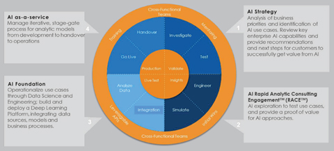
Figure 9.26 A Generalized Framework for AI and Deep Learning–Based Analytics
Summary
Deep learning is the new label for the contemporary applications of artificial intelligence and machine learning. Large collections of unstructured data sources (the big data phenomenon) along with a new generation of neural network architectures set the stage for deep learning and unprecedented promises that it brought alone. The largest data-driven companies including Google, Facebook, Twitter, LinkedIn, Apple, Microsoft, and other are investing millions of dollars into this and related technologies, and making their finding publicly accessible to foster community-based crowed-sourced development projects.
This chapter starts with a clear definition of what deep learning is where it came from. Since the current practice of deep learning relies on artificial neural networks, before delving into the deep learning specific, fundamental concepts are explained early in the chapter. The two popular deep learning architectures, namely CNN and RNN/LSTM are explained, and related community projects and freely accessible class libraries are presented. Also included in the chapter is a brief coverage of cognitive computing and its concepts and applications.
References
Abadi, M., P. Barham, J. Chen, Z. Chen, A. Davis, J. Dean, … M. Isard. (2016). “TensorFlow: A System for Large-Scale Machine Learning.” OSDI, 16, pp. 265–283.
Bahdanau, D., K. Cho, & Y. Bengio. (2014). “Neural Machine Translation by Jointly Learning to Align and Translate.” ArXiv Preprint ArXiv:1409.0473.
Bengio, Y. (2009). “Learning Deep Architectures for AI.” Foundations and Trends® in Machine Learning, 2(1), pp. 1–127.
Bergstra, J., O. Breuleux, F. Bastien, P. Lamblin, R. Pascanu, G. Desjardins, & Y. Bengio. (2010). “Theano: A CPU and GPU Math Compiler in Python.” Proceedings of the Ninth Python in Science Conference, Vol. 1.
Cognitive Computing Consortium (CCC). (2018). https://cognitivecomputingconsortium.com/resources/cognitive-computing-defined/#1467829079735-c0934399-599a (accessed July 2018).
Chen, T., M. Li, Y. Li, M. Lin, N. Wang, M. Wang, … Z. Zhang. (2015). “Mxnet: A Flexible and Efficient Machine Learning Library for Heterogeneous Distributed Systems.” ArXiv Preprint ArXiv:1512.01274.
Collobert, R., K. Kavukcuoglu, & C. Farabet. (2011). “Torch7: A Matlab-like Environment for Machine Learning.” BigLearn, NIPS workshop.
Cybenko, G. (1989). “Approximation by Superpositions of a Sigmoidal Function.” Mathematics of Control, Signals and Systems, 2(4), 303–314.
Goodfellow, I., Y. Bengio, & A. Courville. (2016). “Deep Learning.” Cambridge, MA: MIT Press.
Goodfellow, I. J., D. Warde-Farley, P. Lamblin, V. Dumoulin, M. Mirza, R. Pascanu, … Y. Bengio. (2013). “Pylearn2: A Machine Learning Research Library.” ArXiv Preprint ArXiv:1309.4214.
Graves, A. (2013). “Generating Sequences with Recurrent Neural Networks.” ArXiv Preprint ArXiv:1309.0850.
Graves, A., & N. Jaitly. (2014). “Towards End-to-End Speech Recognition with Recurrent Neural Networks.” Proceedings on International Conference on Machine Learning, pp. 1764–1772.
Gualtieri, M. (2017). “Cognitive Search Is the AI Version of Enterprise Search, Forrester.” go.forrester.com/blogs/17-06-12-cognitive_search_is_the_ai_version_of_enterprise_search/ (accessed July 2018).
Haykin, S. S. (2009). Neural Networks and Learning Machines, 3rd ed. Upper Saddle River, NJ: Prentice Hall.
He, K., X. Zhang, S. Ren, & J. Sun. (2015). “Delving Deep into Rectifiers: Surpassing Human-Level Performance on Imagenet Classification.” Proceedings of the IEEE International Conference on Computer Vision, pp. 1026–1034.
Hinton, G. E., S. Osindero, & Y.-W. Teh, (2006). “A Fast Learning Algorithm for Deep Belief Nets.” Neural Computation, 18(7), 1527–1554.
Hochreiter, S., & J. Schmidhuber (1997). “Long Short-Term Memory.” Neural Computation, 9(8), 1735–1780.
Hornik, K. (1991). “Approximation Capabilities of Multilayer Feedforward Networks.” Neural Networks, 4(2), 251–257.
Jia, Y. (2013). “Caffe: An Open Source Convolutional Architecture for Fast Feature Embedding.” http://Goo.Gl/Fo9YO9.
Keysers, D., T. Deselaers, H. A. Rowley, L.-L. Wang, & V. Carbune. (2017). “Multi-Language Online Handwriting Recognition.” IEEE Transactions on Pattern Analysis and Machine Intelligence, 39(6), pp. 1180–1194.
Krizhevsky, A., I. Sutskever, & G. Hinton. (2012). “Imagenet Classification with Deep Convolutional Neural Networks.” Advances in Neural Information Processing Systems, pp. 1097–1105S.
LeCun, Y., B. Boser, J. S. Denker, D. Henderson, R. E. Howard, W. Hubbard, & L. D. Jackel. (1989). “Backpropagation Applied to Handwritten ZIP Code Recognition.” Neural Computation, 1(4), 541–551.
Liang, X., X. Shen, J. Feng, L. Lin, & S. Yan. (2016). “Semantic Object Parsing with Graph lstm.” European Conference on Computer Vision.New York, NY: Springer, pp. 125–143.
Mahajan, D., R. Girshick, V. Ramanathan, M. Paluri, & L. van der Maaten. (2018). “Advancing State-of-the-Art Image Recognition with Deep Learning on Hashtags.” https://code.facebook.com/posts/1700437286678763/advancing-state-of-the-art-image-recognition-with-deep-learning-on-hashtags/.
Mikolov, T., K. Chen, G. Corrado, & J. Dean. (2013). “Efficient Estimation of Word Representations in Vector Space.” ArXiv Preprint ArXiv:1301.3781.
Mikolov, T., I. Sutskever, K. Chen, G. S. Corrado, & J. Dean. (2013). “Distributed Representations of Words and Phrases and Their Compositionality” Advances in Neural Information Processing Systems, pp. 3111–3119.
Principe, J. C., N. R. Euliano, and W. C. Lefebvre. (2000). Neural and Adaptive Systems: Fundamentals Through Simulations. New York: Wiley.
Reynolds, H., & S. Feldman. (2014, July/August). “Cognitive Computing: Beyond the Hype.” KM World, 23(7), p. 21.
Rumelhart, D. E., G. E Hinton, & R. J. Williams. (1986). “Learning Representations by Back-Propagating Errors.” Nature, 323(6088), pp. 533.
Russakovsky, O., J. Deng, H. Su, J. Krause, S. Satheesh, S. Ma, & M. Bernstein. (2015). “Imagenet Large Scale Visual Recognition Challenge.” International Journal of Computer Vision, 115(3), 211–252.
Sato, K., C. Young, & D. Patterson. (2017). “An In-Depth Look at Google’s First Tensor Processing Unit (TPU).” https://cloud.google.com/blog/big-data/2017/05/an-in-depth-look-at-googles-first-tensor-processing-unit-tpu.
Sutskever, I., O. Vinyals, & Q. V. Le. (2014). “Sequence to Sequence Learning with Neural Networks. Advances in Neural Information Processing Systems, pp. 3104–3112.
Teradata Case Study. (2020). “Danske Bank Fights Fraud with Deep Learning and AI.” https://www.teradata.com/Resources/Case-Studies/Danske-Bank-Fight-Fraud-With-Deep-Learning-and-AI (accessed August 2020).
Ung, G. M. (2016, May). “Google’s Tensor Processing Unit Could Advance Moore’s Law 7 Years into the Future.” PCWorld. https://pcworld.com/article/3072256/google-io/googles-tensor-processing-unit-said-to-advance-moores-law-seven-years-into-the-future.html.
Vinyals, O., A. Toshev, S. Bengio, & D. Erhan. (2015). “Show and Tell: A Neural Image Caption Generator.” Proceedings of the IEEE Conference on Computer Vision and Pattern Recognition (CVPR), pp. 3156–3164.
Vinyals, O., A. Toshev, S. Bengio, & D. Erhan (2017). “Show and Tell: Lessons Learned from the 2015 MSCOCO Image Captioning Challenge.” Proceedings of the IEEE Transactions on Pattern Analysis and Machine Intelligence, 39(4), 652–663.
Zhou, Y.-T., R. Chellappa, A. Vaid, & B. K. Jenkins. (1988). “Image Restoration Using a Neural Network.” IEEE Transactions on Acoustics, Speech, and Signal Processing, 36(7), pp. 1141–1151.