Chapter 5
Algorithms for Predictive Analytics
Predictive analytics algorithms are mostly derived from either traditional statistical methods or from contemporary machine learning techniques. While statistical methods are well established and theoretically sound, machine learning techniques are more accurate, informatics, and actionable/practical (according to a wealth of comparative studies published in the literature). The statistical methods that made the biggest impact in the evolution of predictive analytics and data mining include discriminant analysis, linear regression, and logistic regression. The most popular machine learning techniques used in numerous successful predictive analytics projects include decision trees, k-nearest neighbor, artificial neural networks, and support vector machines. All of these machine learning techniques can handle both classification- as well as regression- type prediction problems. Often, they are applied to complex prediction problems where other, more traditional, techniques are not capable of producing satisfactory results.
Because of the popularity of machine learning techniques in the predictive analytics literature, in this chapter, we explain some of the most common ones in just about enough detail without getting too technical or algorithmic. We also briefly explain the previously mentioned statistical techniques (i.e., linear and logistic regression, and time series analysis) to provide a balanced coverage of the algorithmic spectrum of predictive analytics.
Naïve Bayes
Naïve Bayes is a simple probability-based classification method derived from the well-known Bayes theorem. The method requires output variable to have nominal/categorical values. Although the input variables can be a mix of numeric and nominal types, the numeric output variable needs to be discretized via some type of binning method before it can be used in Naïve Bayes classifier. The word “Naïve” comes from its strong, somewhat unrealistic assumption of independence among the input variables. Simply put, a naive Bayes classifier assumes that the input variables do not depend on each other, and the presence (or absence) of a particular variable in the mix of the predictors does not have anything to do with the presence or absence of any other variables.
Naive Bayes classification models can be developed very efficiently (rather rapidly with very little computational effort) and effectively (quite accurately) in a supervised machine learning environment. That is, using a set of training data (not necessarily very large) the parameters for Naïve Bayes classification models can be obtained using the maximum likelihood method. In other words, because of the independence assumption, we can develop Naïve Bayes models without strictly complying with all of the rules and requirements of Bayes theorem. First let us review the Bayes theorem.
Bayes Theorem
In order to appreciate Naïve Bayes classification method, one would need to understand the basic definition of Bayes theorem and the exact Bayes classifier (the one without the strong “Naïve” independence assumption). Bayes theorem (also called Bayes Rule), named after the British mathematician Thomas Bayes (1701–1761), is a mathematical formula for determining conditional probabilities (the formula is given below). In this formula, Y denotes the hypothesis and X denoted the data/evidence. This vastly popular theorem/rule provides a way to revise/improve prediction probabilities by using additional evidence.
The following formula shows the relationship between the probabilities of two events Y and X. P(Y) is the prior probability of Y. It is “prior” in the sense that it does not take into account any information about X. P(Y∣X) is the conditional probability of Y, given X. It is also called the posterior probability because it is derived from (or depends upon) the specified value of X. P(X∣Y) is the conditional probability of X given Y. It is also called the likelihood. P(X) is the prior probability of X, which is also called the evidence, and acts as the normalizing constant.
![]()
P(Y∣X): Posterior Probability of Y Given X
P(X∣Y): Conditional Probability of X Given Y (Lieklihood)
P(Y): Pior Probability of Y
P(X): Prior Probability of X (Evidence, or Unconditional Probability of X)
To numerically illustrate these formulas let us look at a simple example. Based on the weather report, we know that there is a 40% chance of rain on Saturday. From the historical data, we also know that if it rains on Saturday, with a 10% chance it will rain on Sunday; and if doesn’t rain on Saturday, with an 80% chance it will rain on Sunday. Let us say that “Raining on Sunday” is event Y, and “Raining on Monday” is event X. Based on the description we can write the following:
P(Y) = Probability of Raining on Saturday = 0.40
P(X∣Y) = Probability of it raining on Sunday, if it rained on Saturday = 0.10
P(X) = Probability of Raining on Monday = Sum of the probability of “Raining on Saturday and Raining on Sunday” and “Not raining on Saturday and raining on Sunday” = 0.40 * 0.10 + 0.60 * 0.80 = 0.52
Now if we were to calculate the probability for “It rained on Saturday?” given that it “Rained on Sunday,” we would use Bayes’ theorem. It would allow us to calculate the probability of an earlier event, given the result of a later event.
![]()
Therefore, in this example, if it rained on Sunday, there’s a 7.69% chance it rained on Saturday.
Naïve Bayes Classifier
Bayes classifier uses Bayes theorem without the simplifying strong independence assumption. In a classification type prediction problem Bayes classifier works as follow: Given a new sample to classify, it finds all other samples exactly like it (i.e., all predictor variables having the same values as the sample being classified); determines the class labels that they all belong to; classifies the new sample into the most representative class. If none of the samples has the exact value match with the new class, then the classifier will fail in assigning the new sample into a class label (because it could not find any strong evidence to do so). Here is a very simple example. Using Bayes classifier, we are to decide whether to play golf (Yes or No) for the following situation (Outlook is Sunny, Temperature is Hot, Humidity is High, and Windy is No).
Process of Developing Naïve Bayes Classifier
Similar to other machine learning methods, Naïve Bayes employs a two-phase model development and scoring/deployment process: (1) training, where the model/parameters are estimated, and (2) testing, where the classification/perdition is performed on new cases. The process is described in the following sections.
Training Phase
The steps involved in the training phase
Step 1. Obtain the data, clean the data, and organize it in a flat file format (i.e., columns as variables and rows as cases)
Step 2. Make sure that the variables are a nominal; if not (that is, if any one of the variables is numeric/continuous) then the numeric variables need to go through a data transformation (i.e., converting the numerical variable into nominal types by using discretization, such as binning)
Step 3. Calculate the prior probability of all class labels for the dependent variable
Step 4. Calculate the likelihood for all predictor variables and their possible values with respect to the dependent variable. In the case of mixed variables types (categorical and continuous), each variables’ likelihood (conditional probability) is estimated with the proper method that apply to the specific variable type. Likelihoods for nominal and numeric predictor variables are calculated as follows:
• For categorical variables, the likelihood (the conditional probability) is estimated as the simple fraction of the training samples for the variable value with respect to the dependent variable.
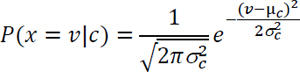
• For numerical variables, the likelihood is calculated by (1) calculating the mean and variance for each predictor variable for each dependent variable value (i.e., class), and then (2) calculating the likelihood using the following formula:
Quite often, the continuous/numerical independent/input variables are discretized (using an appropriate binning method) and then categorical variable estimation method is used to calculate the conditional probabilities (likelihood parameters). If performed properly, this method tends to produce better predicting Naive Bayes models.
Testing Phase
Using the two sets of parameters produced in the Steps 3 and 4 in the training phase, any new sample can be classified into a class label using the following formula:

Since the denominator is constant (the same for all class labels), we can remove it from the formula, leading to the following simpler formula, which is essentially nothing but the joint probability.

Although Naïve Bayes is not very commonly used in predictive analytics project nowadays (due to its relatively poor prediction performance in a wide variety of application domains), one of its extensions, namely Bayesian Network is gaining surprisingly rapid popularity amongst the data scientist in the analytics world.
Nearest Neighbor
Predictive analytics algorithms tend to be highly mathematical and computationally intensive. Two popular ones—artificial neural networks and support vector machines—are involved in overly time-demanding, computationally intensive iterative mathematical derivations. In contrast, the k-nearest neighbor algorithm (k-NN) seems overly simplistic for a competitive prediction method. It is easy to understand (and explain to others) what it does and how it does it. k-NN is a prediction method for classification as well as regression-type prediction problems. k-NN is a type of instance-based learning (or lazy learning) where the function is only approximated locally, and all computations are deferred until the actual prediction.
The k-NN algorithm is among the simplest of all machine learning algorithms. For instance, in classification-type prediction, a case is classified by a majority vote of its neighbors, with the object being assigned to the class most common among its k nearest neighbors (where k is a positive integer). If k = 1, then the case is simply assigned to the class of its nearest neighbor. To illustrate the concept with an example, Figure 5.1 shows a simple two-dimensional space representing the values for the two variables x and y; the star represents a new case (or object), and circles and squares represent known cases (or examples). The task is to assign the new case either to circles or squares, based on its closeness (similarity) to one or the other. If you set the value of k to 1 (k = 1), the assignment should be made to square because the closest example to a star is a square. If you set the value of k to 3 (k = 3), then the assignment should be made to a circle because there are two circles and one square, and hence by simple majority vote rule, the circle gets the assignment of the new case. Similarly, if you set the value of k to 5 (k = 5), then the assignment should be made to the square class. This overly simplified example is meant to illustrate the importance of the value assigned to k.
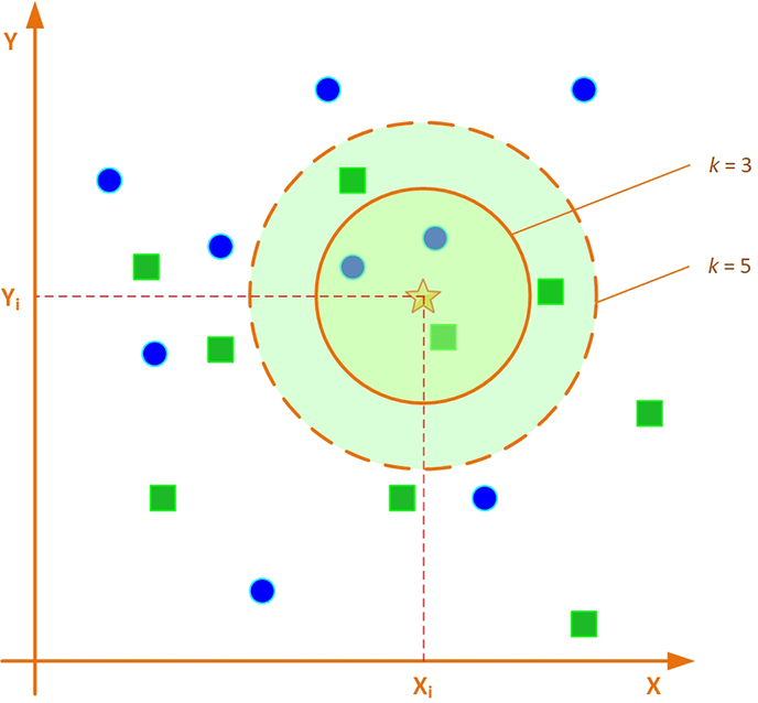
Figure 5.1 The Importance of the Value of k in the k-NN Algorithm
The same method can also be used for regression-type prediction tasks, by simply averaging the values of the k nearest neighbors and assigning that result to the case being predicted. It can be useful to weight the contributions of the neighbors so that the nearer neighbors contribute more to the average than do the more distant ones. A common weighting scheme is to give each neighbor a weight of 1/d, where d is the distance to the neighbor. This scheme is essentially a generalization of linear interpolation.
The neighbors are taken from a set of cases for which the correct classification (or, in the case of regression, the numeric value of the output value) is known. This can be thought of as the training set for the algorithm, even though no explicit training step is required. The k-nearest neighbor algorithm is sensitive to the local structure of the data.
Similarity Measure: The Distance Metric
One of the two critical decisions that an analyst has to make while using k-NN is to determine the similarity measure; the other is to determine the value of k, which is explained below. In the k-NN algorithm, the similarity measure is a mathematically calculable distance metric. Given a new case, k-NN makes predictions based on the outcome of the k neighbors closest in distance to that point. Therefore, to make predictions with k-NN, an analyst needs to define a metric for measuring the distance between the new case and the cases from the examples. One of the most popular choices for measuring this distance is known as Euclidean (Equation 3), which is simply the linear distance between two points in a dimensional space; the other popular one is the rectilinear (a.k.a. city-block or Manhattan distance) (Equation 2). Both of these distance measures are special cases of Minkowski distance (Equation 5.1).
Here is the equation for finding the Minkowski distance:
![]()
where i = (xi1, xi2, ..., xip) and j = (xj1, xj2, ..., xjp) are two p-dimensional data objects (e.g., a new case and an example in the data set), and q is a positive integer.
If q = 1, then d is called Manhattan distance and is found using this equation:
![]()
If q = 2, then d is called Euclidean distance and is found using this equation:
![]()
Obviously, these measures apply only to numerically represented data. What happens with nominal data? There are ways to measure distance for nonnumeric data as well. In the simplest case, for a multivalue nominal variable, if the value of that variable for the new case and the example case is the same, the distance would be zero; otherwise, it would be one. In cases such as text classification, more sophisticated metrics exist, such as the overlap metric (or Hamming distance). Often, the classification accuracy of k-NN can be improved significantly if the distance metric is determined through an experimental design where different metrics are tried and tested to identify the best one for the given problem.
Parameter Selection
The best choice for k depends on the data; generally, larger values of k reduce the effect of noise on the classification (or regression) but also make boundaries between classes less distinct. An “optimal” value of k can be found by using some heuristic techniques, such as cross-validation. The special case where the class is predicted to be the class of the closest training sample (i.e., when k = 1) is called the nearest-neighbor algorithm.
Cross-Validation
Cross-validation is a well-established experimentation technique that can be used to determine optimal values for a set of unknown model parameters. It applies to most, if not all, of the machine learning techniques, where there are a number of model parameters to be determined. The general idea of this experimentation method is to divide the data sample into a number of randomly drawn, disjointed subsamples (i.e., v number of folds). For each potential value of k, the k-NN model is used to make predictions on the vth fold while using the v – 1 folds as the examples, and evaluate the error. The common choice for this error is the root-mean-squared-error (RMSE) for regression-type predictions and percentage of correctly classified instances (i.e., hit rate) for classification-type predictions. This process of testing each fold against the remaining of examples repeats v times. At the end of the v number of cycles, the computed errors are accumulated to yield a goodness measure of the model (i.e., how well the model predicts with the current value of the k). At the end, the k value that produces the smallest overall error is chosen as the optimal value for that problem. Figure 5.2 shows a simple process where training data is used to determine optimal values for k and distance metric, which are then used to predict new incoming cases.

Figure 5.2 The Process of Determining the Optimal Values for the Distance Metric and k
As in the simple example given above, the accuracy of the k-NN algorithm can be significantly different with different values of k. Furthermore, the predictive power of the k-NN algorithm degrades in the presence of noisy, inaccurate, or irrelevant features. Much research effort has been put into feature selection and normalization/scaling to ensure reliable prediction results. A particularly popular approach is the use of evolutionary algorithms (e.g., genetic algorithms) to optimize the set of features included in the k-NN prediction system. In binary (two-class) classification problems, it is helpful to choose an odd number for k to avoid tied votes.
A drawback to the basic majority voting classification in k-NN is that the classes with the more frequent examples tend to dominate the prediction of the new vector, as they tend to come up in the k nearest neighbors when the neighbors are computed due to their large number. One way to overcome this problem is to weigh the classification, taking into account the distance from the test point to each of its k nearest neighbors. Another way to overcome this drawback is to use one level of abstraction in data representation.
The naïve version of the algorithm is easy to implement by computing the distances from the test sample to all stored vectors, but it is computationally intensive, especially when the size of the training set grows. Many nearest-neighbor search algorithms have been proposed over the years; they generally seek to reduce the number of distance evaluations actually performed. Using an appropriate nearest-neighbor search algorithm makes k-NN computationally tractable even for large data sets.
Artificial Neural Networks
Neural networks represent a brain metaphor for information processing. These models are biologically inspired rather than an exact replica of how the brain actually -functions. Neural networks have been shown to be very promising systems in many forecasting and business classification applications due to their ability to “learn” from the data, their nonparametric nature (i.e., no rigid assumptions), and their ability to generalize. Neural computing refers to a pattern-recognition methodology for machine learning. The -resulting model from neural computing is often called an artificial neural -network (ANN) or a neural network. Neural networks have been used in many business -applications for pattern recognition, forecasting, prediction, and classification. Neural network -computing is a key component of any data science and business analytics toolkit. Applications of neural networks abound in finance, marketing, manufacturing, operations, information systems, and so on.
Since we cover neural networks, especially the feed-forward multi-layer perceptron type prediction model-ling specific neural network architecture, in Chapter 6 (which is dedicated to Deep Learning and Cognitive Computing) as a primer to the understanding of Deep Learning and Deep Neural Networks, in this section we provide only a brief introduction to the vast variety of neural network models, methods, and applications.
The human brain possesses bewildering capabilities for information processing and problem solving that modern computers cannot compete with in many aspects. It has been postulated that a model or a system that is enlightened and supported by the results from brain research, with a structure similar to that of biological neural networks, could exhibit similar intelligent functionality. Based on this bottom-up approach, ANN (also known as connectionist models, parallel distributed processing models, neuromorphic -systems, or simply neural net-works) have been developed as biologically inspired and plausible models for various tasks.
Biological neural networks are composed of many massively interconnected-neurons. Each neuron pos-sesses axons and dendrites, fingerlike projections that enable the neuron to communicate with its neighboring neurons by transmitting and receiving electrical and chemical signals. More or less resembling the structure of their biological counterparts, ANN are composed of interconnected, simple processing -elements called artifi-cial neurons. When processing information, the processing elements in an ANN operate concurrently and col-lectively, similar to biological neurons. ANN possess some desirable traits similar to those of biological neural networks, such as the abilities to learn, to self-organize, and to support fault tolerance.
Coming along a winding journey, ANN have been investigated by researchers for more than half a centu-ry. The formal study of ANN began with the pioneering work of McCulloch and Pitts in 1943. Inspired by the results of biological -experiments and -observations, McCulloch and Pitts (1943) introduced a simple model of a binary -artificial neuron that captured some of the functions of biological neurons. Using -information-processing machines to model the brain, McCulloch and Pitts built their neural network model using a large number of interconnected artificial binary -neurons. From these beginnings, neural network research became quite popular in the late 1950s and early 1960s. After a thorough analysis of an early neural network model (called the -perceptron, which used no hidden layer) as well as a pessimistic evaluation of the research poten-tial by Minsky and Papert in 1969, interest in neural networks diminished.
During the past two decades, there has been an exciting resurgence in ANN studies due to the introduc-tion of new network topologies, new activation functions, and new learning algorithms, as well as progress in neuroscience and cognitive science. Advances in theory and methodology have overcome many of the obstacles that hindered neural network research a few decades ago. Evidenced by the appealing results of numerous stud-ies, neural networks are gaining in acceptance and popularity. In addition, the desirable features in neural in-formation processing make neural networks attractive for solving complex problems. ANN have been applied to numerous complex problems in a variety of application settings. The successful use of neural network applica-tions has inspired renewed interest from industry and business. With the emergence of Deep Neural Networks (as part of the rather recent Deep Learning phenomenon) the popularity of neural network (with a “deeper” ar-chitectural representation and much enhanced analytics capabilities), hit an unprecedented height, creating mile-high expectations from this new generation of neural networks. Deep neural networks are covered in detail in Chapter 6.
Biological versus Artificial Neural Networks
The human brain is composed of special cells called neurons. These cells do not die and replenish when a per-son is injured (all other cells reproduce to replace themselves and then die). This phenomenon may explain why humans retain information for an extended period of time and start to lose it when they get old—as the brain cells -gradually start to die. Information storage spans sets of neurons. The brain has anywhere from 50 billion to 150 billion neurons, of which there are more than 100 different kinds. Neurons are -partitioned into groups called networks. Each network contains several thousand highly interconnected neurons. Thus, the brain can be viewed as a collection of neural networks.
The ability to learn and to react to changes in our environment requires -intelligence. The brain and the central nervous system control thinking and intelligent behavior. People who suffer brain damage have difficul-ty learning and reacting to changing environments. Even so, undamaged parts of the brain can often compensate with new learning.
A portion of a network composed of two cells is shown in Figure 5.3. The cell itself includes a nucleus (the central processing portion of the neuron). To the left of cell 1, the dendrites provide input signals to the cell. To the right, the axon sends output signals to cell 2 via the axon terminals. These axon terminals merge with the dendrites of cell 2. Signals can be transmitted unchanged, or they can be altered by synapses. A syn-apse is able to increase or decrease the strength of the connection between neurons and cause excitation or inhi-bition of a subsequent neuron. This is how information is stored in the neural networks.

Figure 5.3 A Biological Neural Network: Two Interconnected Cells/Neurons
An ANN emulates a biological neural network. Neural computing actually uses a very limited set of concepts from biological neural systems. A simple terminology mapping between biological and artificial neural networks is shown in Table 5.1. It is more of an analogy to the human brain than an accurate model of it. Neural concepts usually are implemented as software simulations of the massively parallel processes involved in processing interconnected elements (also called artificial neurons, or neurodes) in a network architecture. The artificial neuron receives inputs analogous to the electrochemical impulses that dendrites of biological neurons receive from other neurons. The output of the artificial neuron corresponds to signals sent from a biological neuron over its axon. These artificial signals can be changed by weights in a manner similar to the physical changes that occur in the synapses (see Figure 5.4).
Table 5.1 Mapping Between Biological and Artificial NNs
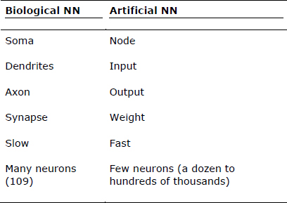
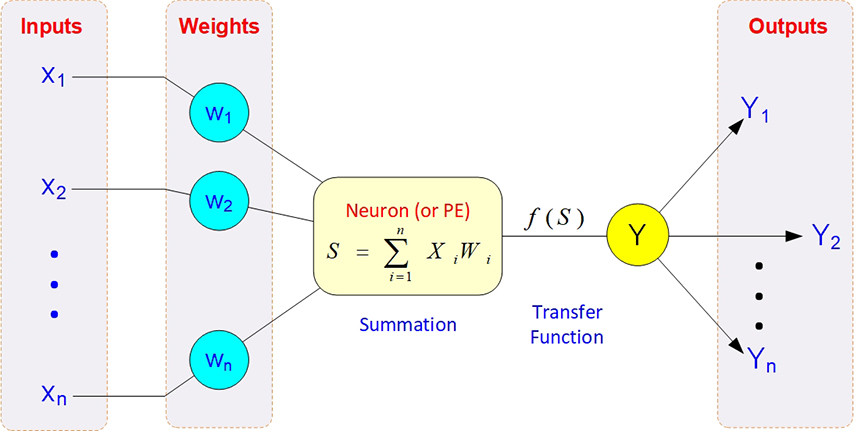
Figure 5.4 Processing Information in an Artificial Neuron
Several ANN paradigms have been proposed for applications in a variety of problem domains. Perhaps the easiest way to differentiate among the various neural models is on the basis of how they structurally emulate the human brain, the way they process information, and how they learn to perform their designated tasks.
Because they are biologically inspired, the main processing elements of a neural network are individual neurons, analogous to the brain’s neurons. These artificial neurons receive information from other neurons or external input stimuli, perform a transformation on the inputs, and then pass on the transformed information to other neurons or external outputs. This is similar to how it is presently thought that the human brain works. Passing information from neuron to neuron can be thought of as a way to activate, or trigger, a response from certain neurons based on the information or stimulus received.
How information is processed by a neural network is inherently a function of its structure. Neural networks can have one or more layers of neurons. These neurons can be highly or fully interconnected, or only certain layers can be connected. Connections between neurons have an associated weight. In essence, the “knowledge” possessed by the network is encapsulated in these interconnection weights. Each neuron calculates a weighted sum of the incoming neuron values, transforms this input, and passes on its neural value as the input to subsequent neurons. Typically, although not always, this input/output transformation process at the individual neuron level is performed in a nonlinear fashion.
Support Vector Machines
Support vector machines (SVMs) are among the most popular machine learning techniques in the recent past, largely because of their superior predictive performance and their theoretical foundation. SVMs are among the supervised learning methods that produce input/output functions from a set of labeled training data. The function between the input and output vectors can be either a classification function (used to assign cases into predefined classes) or a regression function (used to estimate the continuous numeric value of the desired output). For classification, nonlinear kernel functions are often used to transform the input data (naturally representing highly complex nonlinear relationships) to a high dimensional feature space in which the input data becomes linearly separable. Then, the maximum-margin hyperplanes are constructed to optimally separate the output classes from each other in the training data.
For a given classification-type prediction problem, generally speaking, many linear classifiers (hyperplanes) can separate the data into multiple subsections, each representing one of the classes (see Figure 5.5a, where the two classes are represented with circles [•] and squares [□]). However, only one hyperplane achieves the maximum separation between the classes (see Figure 5.5b, where the hyperplane and the two maximum-margin hyperplanes are separating the two classes).
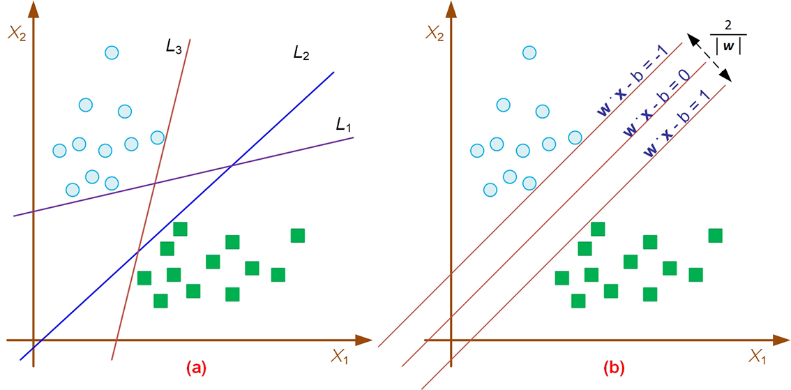
Figure 5.5 Separation of the Two Classes with Support Vector Machines
Data used in SVMs may have more than two dimensions (i.e., two distinct classes). In that case, we would be interested in separating data using n – 1 dimensional hyperplanes, where n is the number of dimensions (i.e., class labels). This may be seen as a typical form of linear classifier, where we are interested in finding n – 1 hyperplanes so that the distance from the hyperplanes to the nearest data points are maximized. The assumption is that the larger the margin or distance between these parallel hyperplanes, the better the generalization power of the classifier (i.e., prediction power of the SVM model). If such hyperplanes exist, they can be mathematically represented using quadratic optimization modeling. These hyperplanes are known as the maximum-margin hyperplanes, and a linear classifier is known as a maximum-margin classifier.
In addition to their solid mathematical foundation in statistical learning theory, SVMs have also demonstrated highly competitive performance in numerous real-world prediction problems, such as medical diagnosis, bioinformatics, face/voice recognition, demand forecasting, image processing, and text mining, which has established SVMs as one of the most popular analytics tools for knowledge discovery and data mining. Similarly to artificial neural networks, SVMs can be used to approximate any multivariate function to any desired degree of accuracy. Therefore, they are of particular interest in modeling highly nonlinear, complex problems, systems, and processes.
The Process of Building SVM Models
Recently, using support vector machines has become a popular technique for classification-type problems because of their predictive accuracy and self-expandability. Even though people consider them easier to use than artificial neural networks, users who are not familiar with the intricacies of SVMs often get unsatisfactory results. In this section we provide a simple process-based approach to model building with and use of SVMs that is likely to produce good results. A pictorial representation of the three-step process is given in Figure 5.6.
Following are short descriptions of the steps in this process.
Step 1: Preprocess the Data
Because real-world data is anything but perfect, a data mining analyst needs to do the due diligence to scrub and transform the data for SVM. As is the case with any other data mining methods and algorithms, this step is likely to be the most time-demanding and least enjoyable, yet most essential, part of working with SVMs. Some of the tasks in this step include handling missing, incomplete, and noisy values and numerisizing, normalizing, and standardizing the data:
• Numerisizing the data. SVMs require that each data instance be represented as a vector of real numbers. Hence, if there are categorical attributes, an analyst has to first convert them into numeric data. A common recommendation is to use m pseudo binary variables to represent an m-class attribute (where m ≥ 3). In practice, only one of the m variables assumes the value of 1, and others assume the value of 0, based on the actual class of the case; this is also called 1-of-m representation. For example, a three-category attribute such as {red, green, blue} can be represented as (0,0,1), (0,1,0), and (1,0,0).
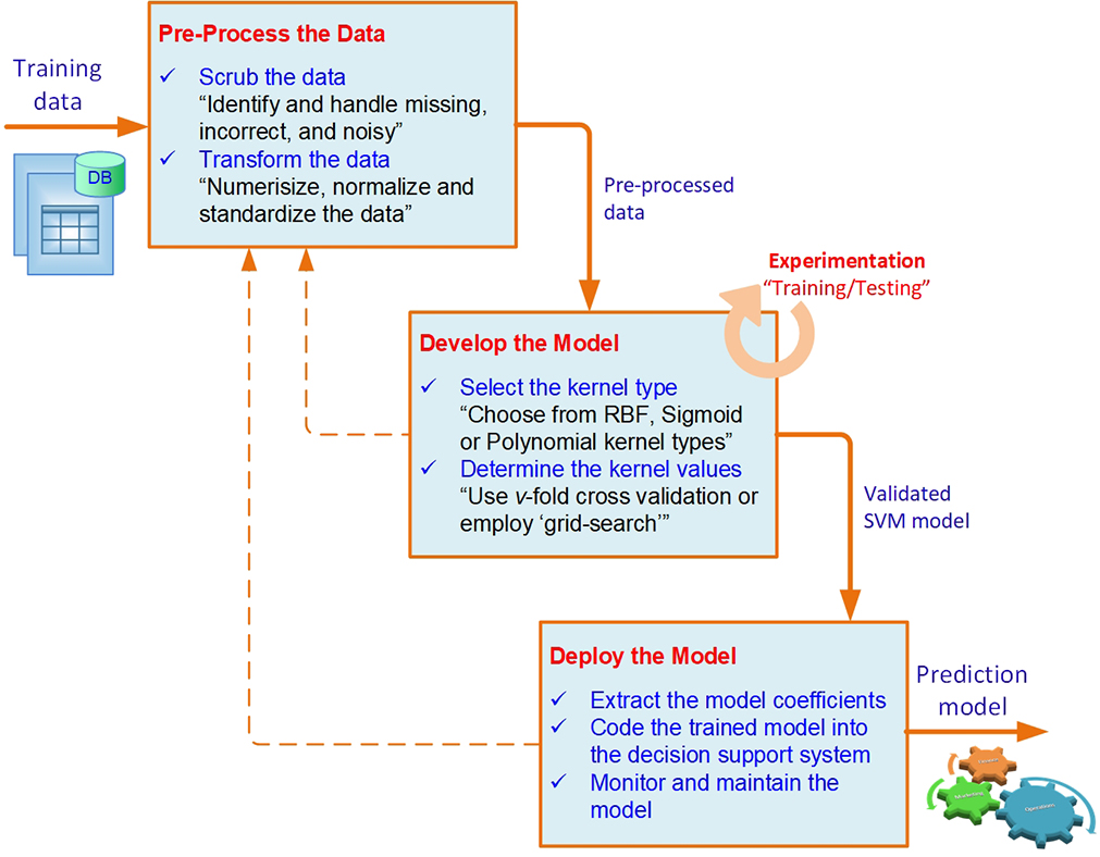
Figure 5.6 A Simple Process for Developing and Using SVM Models
• Normalizing the data. As is the case with artificial neural networks, SVMs also require normalization and/or scaling of numeric values. The main advantage of normalization is to avoid having attributes in greater numeric ranges dominate those in smaller numeric ranges. Another advantage is that it helps perform numeric calculations during the iterative process of model building. Because kernel values usually depend on the inner products of feature vectors (e.g., the linear kernel, the polynomial kernel), large attribute values might slow the training process. The usual recommendation is to normalize each attribute to the range [-1, +1] or [0, 1]. Of course, an analyst has to use the same normalization method to scale testing data before testing.
Step 2: Develop the Model
Once the data is preprocessed, the model building step starts. Compared to the other two steps, this is the most enjoyable part of the process, where the prediction model comes alive. Because SVM has a number of parameter options, the process requires a lengthy process of determining the optimal combination of those parameters for the best possible performance. The most important of those parameters are the kernel type and consequently kernel-related subparameters.
There are four common kernels, and an analyst must decide which one to use (or whether to try them all, one at a time, using a simple experimental design approach). Once the kernel type is selected, the analyst needs to select the value of penalty parameter C and the kernel parameters. Generally speaking, RBF is a reasonable first choice for the kernel type. The RBF kernel aims to nonlinearly map data into a higher dimensional space, and this (unlike with a linear kernel) handles the cases where the relationship between input and output vectors is highly nonlinear. Besides, the linear kernel is just a special case of the RBF kernel. There are two parameters to choose for RBF kernels: C and y. It is not known beforehand which C and y are the best for a given prediction problem; therefore, some kind of parameter search method needs to be used. The goal for the search is to identify optimal values for C and y so that the classifier can accurately predict unknown data (i.e., testing data). The two most commonly used search methods are cross-validation and grid search.
Step 3: Deploy the Model
Once an optimal SVM prediction model is developed, the next step is to integrate it into the decision support system. For that, there are two options: (1) converting the model into a computational object (e.g., a Web service, a Java Bean, or a COM object) that takes the input parameter values and provides output prediction or (2) extracting the model coefficients and integrating them directly into the decision support system. The SVM models are useful (i.e., accurate and actionable) only if the behavior of the underlying domain stays the same. For some reason, if the behavior changes, so does the accuracy of the model. Therefore, it’s important to continuously assess the performance of the models and decide when they are no longer accurate and, hence, need to be retrained.
Support Vector Machines Versus Artificial Neural Networks
Even though some people characterize SVMs as a special case of ANNs, most recognize these as two competing machine learning techniques with different qualities. Let’s look at a few points that help SVMs stand out against ANNs. Historically, the development of ANNs followed a heuristic path, with applications and extensive experimentation preceding theory. In contrast, the development of SVMs involved sound statistical learning theory first, followed by implementation and experiments. A significant advantage of SVMs is that while ANNs may suffer from multiple local minima, the solutions to SVMs are global and unique. Two more advantages of SVMs are that they have simple geometric interpretations and give sparse solutions. The reason that SVMs often outperform ANNs in practice is that they successfully deal with the “overfitting” problem, which is a big issue with ANNs.
Besides the above-mentioned advantages of SVMs (from a practical point of view), they also have some limitations. An important issue that is not entirely solved is the selection of the kernel type and kernel function parameters. Other, perhaps more important, limitations of SVMs are the speed and size, both in training and testing cycles. Model building with SVMs involves complex and time-demanding calculations. From a practical point of view, perhaps the most serious problems with SVMs are the high algorithmic complexity and extensive memory requirements of the required quadratic programming in large-scale tasks. Despite these limitations, because SVMs are based on a sound theoretical foundation and the solutions they produce are global and unique in nature (as opposed to getting stuck in suboptimal alternatives as local minima do), today’s SVMs are some of the most popular prediction modeling techniques in the data mining arena. Their use and popularity will only increase as the popular commercial data mining tools start to incorporate them into their modeling arsenals.
Linear Regression
Regression, especially linear regression, is perhaps the most widely used analysis technique in statistics. Historically speaking, the roots of regression date back to the 1920s and 1930s, to the early work on inherited characteristics of sweet peas by Sir Francis Galton and subsequently Karl Pearson. Since then, regression has become the statistical technique for characterization of relationships between explanatory (input) variable(s) and response (output) variable(s).
As popular as it is, regression is essentially a relatively simple statistical technique to model the dependence of a variable (response or output variable) on one (or more) explanatory (input) variables. Once identified, this relationship between the variables can be formally represented as a linear/additive function or equation. As is the case with many other modeling techniques, regression aims to capture the functional relationship between and among the characteristics of the real world and describe this relationship with a mathematical model, which may then be used to discover and understand the complexities of reality—explore and explain relationships or forecast future occurrences.
Regression can be used for two different purposes: hypothesis testing—investigating potential relationships between different variables—and prediction/forecasting—estimating values of response variables based on one or more explanatory variables. These two uses are not mutually exclusive. The explanatory power of regression is also the foundation of its prediction ability. In hypothesis testing (theory building), regression analysis can reveal the existence and strength and the directions of relationships between a number of explanatory variables (often represented with xi) and the response variable (often represented with y). In prediction, regression identifies additive mathematical relationships (in the form of an equation) between one or more explanatory variables and a response variable. Once determined, this equation can be used to forecast the values of response variable for a given set of values of the explanatory variables.
Correlation versus Regression
Because regression analysis originated in correlation studies, and because both methods attempt to describe the association between two (or more) variables, these two terms are often confused by professionals and even by scientists. Correlation makes no a priovri assumption as to whether one variable is dependent on the other(s) and is not concerned with the relationship between variables; instead, it gives an estimate about the degree of association between the variables. On the other hand, regression attempts to describe the dependence of a response variable on one or more explanatory variables, where it implicitly assumes that there is a one-way causal effect from the explanatory variables to the response variable, regardless of whether the path of effect is direct or indirect. Also, whereas correlation is interested in low-level relationships between two variables, regression is concerned with the relationships between all explanatory variables and the response variable.
Simple versus Multiple Regression
If a regression equation is built between one response variable and one explanatory variable, then it is called simple regression. For instance, the regression equation built to predict or explain the relationship between the height of a person (explanatory variable) and the weight of a person (response variable) is a good example of simple regression. Multiple regression is an extension of simple regression in which there are multiple explanatory variables. For instance, in the previous example, if we were to include not only the height of a person but also other personal characteristics (e.g., BMI, gender, ethnicity) to predict the weight of the person, then we would be performing multiple regression analysis. In both cases, the relationships between the response variables and the explanatory variables are linear and additive in nature. If the relationships are not linear, then we might want to use one of many other nonlinear regression methods to better capture the relationships between the input and output variables.
How to Develop a Linear Regression Model
To understand the relationship between two variables, the simplest thing to do is to draw a scatter plot, where the y-axis represents the values of the response variable and the x-axis represents the values of the explanatory variable (see Figure 5.7). Such a scatter plot would show the changes in the response variable as a function of the changes in the explanatory variable. In the example shown in Figure 5.7, there seems to be a positive relationship between the two: As the explanatory variable values increase, so does the response variable.
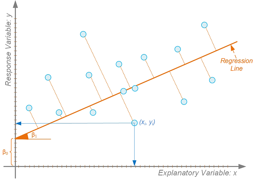
Figure 5.7 A Scatter Plot with a Simple Linear Regression Line
Simple regression analysis aims to find a mathematical representation of this relationship. In reality, it tries to find the signature of a straight line passing right in between the plotted dots (representing the observation/historical data) in such a way that it minimizes the distance between the dots and the line (the predicted values on the theoretical regression line). Several methods/algorithms have been proposed to identify the regression line, and the one that is most commonly used is called the ordinary least squares (OLS) method. The OLS method aims to minimize the sum of squared residuals (i.e., squared vertical distances between the observation and the regression point) and leads to a mathematical expression for the estimated value of the regression line (known as the β parameter). For simple linear regression, the aforementioned relationship between the response variable (y) and the explanatory variable(s) (x) can be shown as a simple equation, as follows:
y = β0 + β1x
In this equation, β0 is called the intercept, and β1 is called the slope. Once OLS determines the values of these two coefficients, the simple equation can be used to forecast the values of y for given values of x. The sign and the value of β1 also reveal the direction and the strength of the relationship between the two variables.
If the model is of a multiple linear regression type, then more coefficients need to be determined—one for each additional explanatory variable. As the following formula shows, the additional explanatory variable would be multiplied with new βi coefficients and summed together to establish a linear additive representation of the response variable.
![]()
How to Tell Whether a Model Is Good Enough
For a variety of reasons, sometimes models do not do a good job representing reality. Regardless of the number of explanatory variables included, there is always a possibility of not having a good model, and therefore a linear regression model needs to be assessed for its fit (the degree to which it represents the response variable). In the simplest sense, a well-fitting regression model results in predicted values close to the observed data values. For the numeric assessment, three statistical measures are often used in evaluating the fit of a regression model. R2 (R-squared), the overall F-test, and the root mean square error (RMSE). All three of these measures are based on sums of square errors (how far the data is from the mean and how far the data is from the model’s predicted values). Different combinations of these two values provide different information about how the regression model compares to the mean model.
Of the three, R2 has the most useful and understandable meaning because of its intuitive scale. The value of R2 ranges from 0 to 1 (corresponding to the amount of variability, expressed as a percentage), with 0 indicating that the relationship and the prediction power of the proposed model is not good and 1 indicating that the proposed model is a perfect fit that produces exact predictions (which is almost never the case). Good R2 values usually come close to 1, and the closeness is a matter of the phenomenon being modeled; for example, while an R2 value of 0.3 for a linear regression model in social science may be considered good enough, an R2 value of 0.7 in engineering might not be considered a good fit. Improvement in the regression model can be achieved by adding more explanatory variables, taking some of the variables out of the model, or using different data transformation techniques, which would result in comparative increases in an R2 value.
Figure 5.8 shows the process flow involved in developing regression models. As shown in the figure, the model development task is followed by model assessment. Model assessment involves assessing the fit of the model and also, because of restrictive assumptions with which linear models have to comply, it also involves examining the validity of the model.

Figure 5.8 Process Flow for Developing Regression Models
The Most Important Assumptions in Linear Regression
Even though they are still the top choice of many data analysis (both for explanatory as well as predictive modeling purposes), linear regression models suffer from several highly restrictive assumptions. The validity of a linear model depends on its ability to comply with these assumptions. Here are the most common assumptions:
• Linearity. This assumption states that the relationship between the response variable and the explanatory variables are linear. That is, the expected value of the response variable is a straight-line function of each explanatory variable, while holding all other explanatory variables fixed. Also, the slope of the line does not depend on the values of the other variables. This implies that the effects of different explanatory variables on the expected value of the response variable are additive in nature.
• Independence (of errors). This assumption states that the errors of the response variable are uncorrelated with each other. This independence of the errors is weaker than actual statistical independence, which is a stronger condition and is often not needed for linear regression analysis.
• Normality (of errors). This assumption states that the errors of the response variable are normally distributed. That is, they are supposed to be totally random and should not represent any nonrandom patterns.
• Constant variance (of errors). This assumption, also called homoscedasticity, states that the response variables must have the same variance in their error, regardless of the values of the explanatory variables. In practice, this assumption is invalid if the response variable varies over a wide enough range or scale.
• Multicollinearity. This assumption states that the explanatory variables are not correlated (i.e., do not replicate the same but provide a different perspective of the information needed for the model). Multicollinearity can be triggered by having two or more perfectly correlated explanatory variables present in the model (e.g., if the same explanatory variable is mistakenly included in the model twice, one with a slight transformation of the same variable). A correlation-based data assessment usually catches this error.
Statistical techniques have been developed to identify the violation of these assumptions, and several techniques have been created to mitigate them. A data modeler needs to be aware of the existence of these assumptions and put in place a way to assess models to make sure they are compliant with the assumptions they are built on.
Logistic Regression
Logistic regression is a very popular, statistically sound, probability-based classification algorithm that employs supervised learning. It was developed in the 1940s as a complement to linear regression and linear discriminant analysis methods. It has been used extensively in numerous disciplines, including the medical and social science fields. Logistic regression is similar to linear regression in that it also aims to regress to a mathematical function that explains the relationship between the response variable and the explanatory variables, using a sample of past observations (training data). It differs from linear regression on one major point: Its output (response variable) is a class as opposed to a numeric variable. That is, whereas linear regression is used to estimate a continuous numeric variable, logistic regression is used to classify a categorical variable. Even though the original form of logistic regression was developed for a binary output variable (e.g., 1/0, yes/no, pass/fail, accept/reject), the present-day modified version is capable of predicting multiple-class output variables (i.e., multinomial logistic regression). If there is only one predictor variable and one predicted variable, the method is called simple logistic regression; this is similar to using the term simple linear regression for a linear regression model with only one independent variable.
In predictive analytics, logistic regression models are used to develop probabilistic models between one or more explanatory or predictor variables (which may be a mix of both continuous and categorical variables) and a class or response variable (which may be binomial/binary or multinomial/multiple-class variables). Unlike ordinary linear regression, logistic regression is used for predicting categorical (often a binary) outcomes of the response variable—treating the response variable as the outcome of a Bernoulli trial. Therefore, logistic regression takes the natural logarithm of the odds of the response variable to create a continuous criterion as a transformed version of the response variable. Thus the logit transformation is referred to as the link function in logistic regression; even though the response variable in logistic regression is categorical or binomial, the logit is the continuous criterion on which linear regression is conducted.
Figure 5.9 shows a logistic regression function where the odds are represented on the x-axis (i.e., a linear function of the independent variables), and the probabilistic outcome is shown on the y-axis (i.e., response variable values change between 0 and 1).
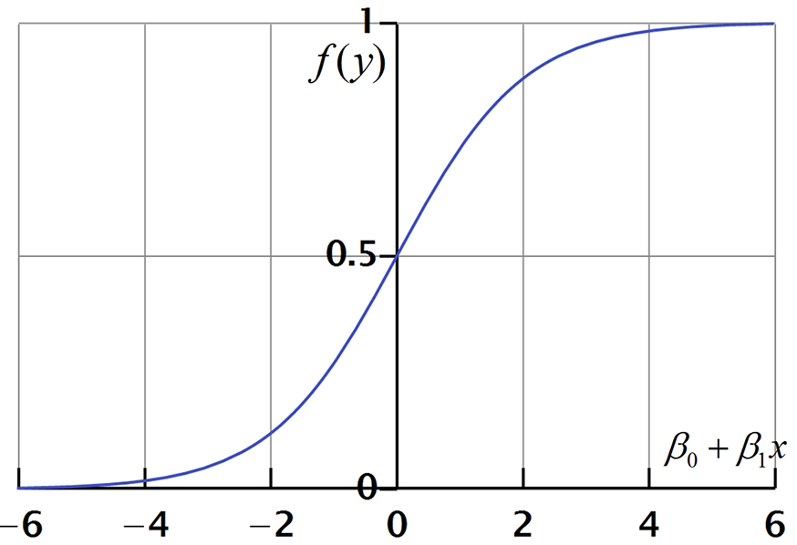
Figure 5.9 The Logistic Function
The logistic function, which is f(y) in Figure 5.9, is the core of logistic regression, which can only take values between 0 and 1. The following equation is a simple mathematical representation of this function:
The logistic regression coefficients (the βs) are usually estimated using the maximum-likelihood estimation method. Unlike with linear regression with normally distributed residuals, it is not possible to find a closed-form expression for the coefficient values that maximizes the likelihood function, so an iterative process must be used instead. This process begins with a tentative starting solution and then revises the parameters slightly to see if the solution can be improved; it repeats this iterative revision until no improvement can be achieved or the improvements are very minimal, at which point the process is said to have completed or converged.
Time-Series Forecasting
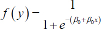
Sometimes the variable of interest (i.e., the response variable) may not have distinctly identifiable explanatory variables, or there may be too many of them in a highly complex relationship. In such cases, if the data is available in the desired format, a prediction model, called a time-series forecast, can be developed. A time series is a sequence of data points of the variable of interest, measured and represented at successive points in time and spaced at uniform time intervals. Examples of time series include monthly rain volumes in a geographic area, the daily closing value of the stock market indices, and daily sales totals for a grocery store. Often, time series are visualized using a line chart. Figure 5.10 shows an example of a time series of sales volumes for the years 2008 through 2012, on a quarterly basis.
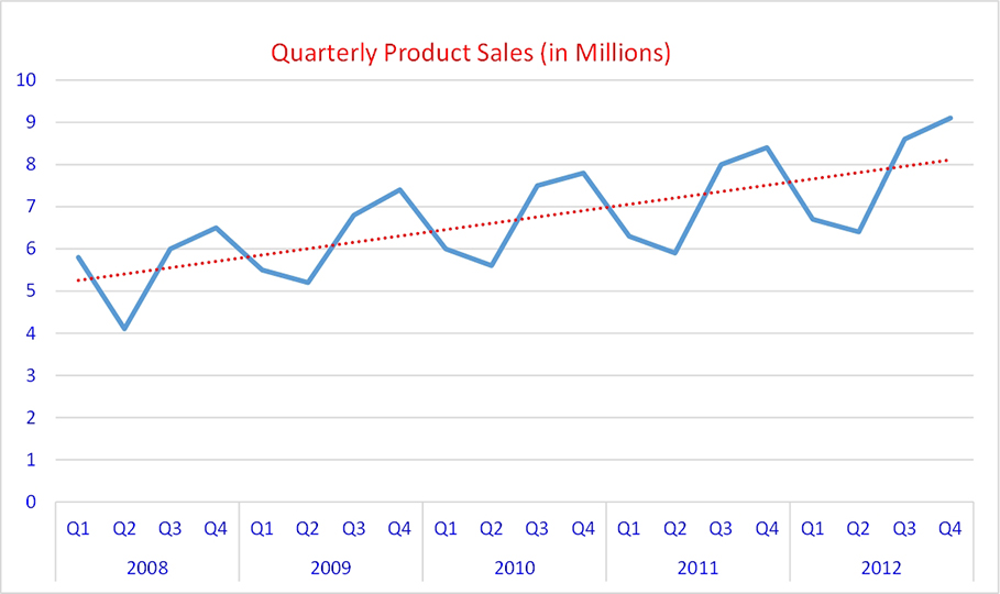
Figure 5.10 Sample Time-Series Data on Quarterly Sales Volumes
Time-series forecasting involves using a mathematical model to predict future values of the variable of interest, based on previously observed values. Time-series plots or charts look very similar to simple linear regression scatter plots in that there are two variables: the response variable and the time variable. Beyond this similarity, there is hardly any other commonality between the two. While regression analysis is often used in testing theories to see if current values of one or more explanatory variables explain (and hence predict) the response variable, time-series models are focused on extrapolating the time-varying behavior to estimate future values.
Time-series forecasting assumes that all the explanatory variables are aggregated and consumed in the response variable’s time-variant behavior. Therefore, capturing time-variant behavior is a way to predict the future values of the response variable. To do that, the pattern is analyzed and decomposed into its main components: random variations, time trends, and seasonal cycles. The time-series example shown in Figure 5.10 illustrates all these distinct patterns.
The techniques used to develop time-series forecasts ranges from very simple (e.g., the naïve forecast which suggests that today’s forecast is the same as yesterday’s actual) to very complex (e.g., ARIMA, which combines autoregressive and moving average patterns in data). The most popular techniques are perhaps the averaging methods that include simple averages, moving averages, weighted moving averages, and exponential smoothing. Many of these techniques also have advanced versions where seasonality and trend can also be taken into account for better and more accurate forecasting. The accuracy of a method is usually assessed by computing its error (i.e., calculated deviation between actuals and forecasts for the past observations) via mean absolute error (MAE), mean squared error (MSE), or mean absolute percent error (MAPE). Even though they all use the same core error measure, these three assessment methods emphasize different aspects of the error, some panelizing larger errors more so than the others.
Application Example: Data Mining for Complex Medical Procedures
Health care has become one of the most important issues related to quality of life in the United States and elsewhere around the world. While the demand for health care services is increasing because of the aging population, the supply side is having problems keeping up with the level and quality of service. In order to close the gap, health care systems need to significantly improve their operational effectiveness and efficiency. Effectiveness (doing the right thing, such as diagnosing and treating accurately) and efficiency (doing it the right way, such as using the least resources and time) are the two fundamental pillars on which the health care system can be revived. A promising way to improve health care is to take advantage of predictive modeling techniques along with large and feature-rich data sources (true reflections of medical and health care experiences) to support accurate and timely decision making.
According to the American Heart Association, cardiovascular disease (CVD) is the underlying cause of more than 20% of deaths in the United States. Since 1900, CVD has been the number-one killer every year except 1918, which was the year of the great flu pandemic. CVD kills more people than the next four leading causes of death—cancer, chronic lower respiratory disease, accidents, and diabetes mellitus—combined. More than half of all CVD deaths can be attributed to coronary diseases. Not only does CVD take a huge toll on the personal health and well-being of the population, it is also a great drain on the health care resources in the United States and elsewhere in the world. The direct and indirect costs associated with CVD for a year are estimated to exceed $500 billion. A common surgical procedure to cure a large variant of CVD is called coronary artery bypass grafting (CABG). The cost of a CABG surgery depends on the patient and factors related to the service provider, but the average rate in the United States is between $50,000 and $100,000. As an illustrative example, Delen et al. (2012) carried out an analytics study in which they used various predictive modeling methods to predict the outcome of a CABG surgery, and they applied an information fusion–based sensitivity analysis on the trained models to better understand the importance of the prognostic factors. The main goal was to illustrate that predictive and explanatory analysis of large and feature-rich data sets provides invaluable information for making more efficient and effective decisions in health care.
Research Method
Figure 5.11 shows the model development and testing process Delen et al. used. They employed four different types of prediction models (artificial neural networks, support vector machines, and two types of decision trees, C5 and CART) and went through a large number of experimental runs to calibrate the modeling parameters for each model type. Once the models were developed, then they used the models on the text data set. Finally, the trained models were exposed to a sensitivity analysis procedure to measure the contributions of the variables. Table 5.2 shows the test results for the four different types of prediction models.
Figure 5.11 A Process Map for Training and Testing of the Four Predictive Models
Table 5.2 Prediction Accuracy Results for All Four Model Types, Based on the Test Data Set

Results
In this study, Delen et al. showed the power of data mining in predicting the outcome and in analyzing the prognostic factors of complex medical procedures such as CABG surgery. They showed that using a number of prediction methods (as opposed to only one) in a competitive experimental setting has the potential to produce better predictive as well as explanatory results. Among the four methods they used, SVMs produced the best results, with prediction accuracy of 88% on the test data sample. The information fusion–based sensitivity analysis revealed the ranked importance of the independent variables. Some of the top variables identified in this analysis overlapped with the most important variables identified in previously conducted clinical and biological studies; this confirms the validity and effectiveness of the proposed data mining methodology.
From a managerial standpoint, clinical decision support systems that use the outcomes of data mining studies (such as the ones presented in this case study) are not meant to replace health care managers and/or medical professionals. Rather, they are meant to support them in making accurate and timely decisions to optimally allocate resources in order to increase the quantity and quality of medical services. We still have a long way to go before we will see these decision aids being used extensively in health care practices. Among others, there are behavioral, ethical, and political reasons for the resistance to adopting these tools. Perhaps need and government incentives for better health care systems will expedite their adoption.
Summary
Predictive analytics employs several algorithms, some seemingly too simple while other are more complex, some have its origins in traditional statistics while others have their roots in emergent trends in artificial intelligence and machine learning. The algorithms covered in this chapter include naïve Bayes, k-nearest neighbor, artificial neural networks (only a primer provided herein and the detailed descriptions of neural networks are left to be covered in Chapter 9, within the context of deep learning), support vector machines, linear regression, logistic regression, and time series forecasting.
The goal of the chapter was to provide just about enough information (breadth and depth) about these algorithms (without getting too deep into the theory and mathematical complexities) so that the reader could understand and appreciate how these algorithms really work (i.e., how they do what they do). Knowing the innerworkings of these algorithms, at least at a conceptual level, helps analytics professional and data scientist to make informed and smarter decisions related to the preprocessing of the data, framing of the problem, and creation of the solution methodology. Analogically, one can relate to this phenomenon in the context of a race car driver: having to know how engine works makes a better driver. Although the race car driver is not expected to build or repair the engine, having the understanding of the innerworkings of the engine helps the driver in optimizing its capacity by maximizing its power and productivity.
References
Aizerman, M., E. Braverman, & L. Rozonoer. (1964). “Theoretical Foundations of the Potential Function Method in Pattern Recognition Learning,” Automation and Remote Control, 25: 821–837.
Collins, E., S. Ghosh, & C. L. Scofield. (1988). “An Application of a Multiple Neural Network Learning System to Emulation of Mortgage Underwriting Judgments.” IEEE International Conference on Neural Networks, 2: 459–466.
Das, R., I. Turkoglu, & A. Sengur. (2009). “Effective Diagnosis of Heart Disease Through Neural Networks Ensembles,” Expert Systems with Applications, 36: 7675–7680.
Delen, D., A. Oztekin, & L. Tomak. (2012). “An analytic approach to better understanding and management of coronary surgeries,” Decision Support Systems, 52(3): 698–705.
Delen, D., R. Sharda, & M. Bessonov. (2006). “Identifying Significant Predictors of Injury Severity in Traffic Accidents Using a Series of Artificial Neural Networks,” Accident Analysis and Prevention, 38(3): 434–444.
Delen, D., & E. Sirakaya. (2006). “Determining the Efficacy of Data-Mining Methods in Predicting Gaming Ballot Outcomes,” Journal of Hospitality & Tourism Research, 30(3): 313–332.
Fadlalla, A., & C. Lin. (2001). “An Analysis of the Applications of Neural Networks in Finance,” Interfaces, 31(4).
Haykin, S. S. (2009). Neural Networks and Learning Machines, 3rd ed. Upper Saddle River, NJ: Prentice Hall.
Hill, T., T. Marquez, M. O’Connor, & M. Remus. (1994). “Neural Network Models for Forecasting and Decision Making,” International Journal of Forecasting, 10.
Hopfield, J. (1982). “Neural Networks and Physical Systems with Emergent Collective Computational Abilities,” Proceedings of the National Academy of Science, 79(8).
Liang, T. P. (1992). “A Composite Approach to Automated Knowledge Acquisition,” Management Science, 38(1).
Loeffelholz, B., E. Bednar, & K. W. Bauer. (2009). “Predicting NBA Games Using Neural Networks,” Journal of Quantitative Analysis in Sports, 5(1).
McCulloch, W. S., & W. H. Pitts. (1943). “A Logical Calculus of the Ideas Imminent in Nervous Activity,” Bulletin of Mathematical Biophysics, 5.
Minsky, M., & S. Papert. (1969). Perceptrons. Cambridge, MA: MIT Press.
Piatesky-Shapiro, G. ISR: Microsoft Success Using Neural Network for Direct Marketing, http://kdnuggets.com/news/94/n9.txt (accessed May 2020).
Principe, J. C., N. R. Euliano, & W. C. Lefebvre. (2000). Neural and Adaptive Systems: Fundamentals Through Simulations. New York: Wiley.
Sirakaya, E., D. Delen, & H-S. Choi. (2005). “Forecasting Gaming Referenda,” Annals of Tourism Research, 32(1): 127–149.
Tang, Z., C. de Almieda, & P. Fishwick. (1991). “Time-Series Forecasting Using Neural Networks vs. Box-Jenkins Methodology,” Simulation, 57(5).
Walczak, S., W. E. Pofahi, & R. J. Scorpio. (2002). “A Decision Support Tool for Allocating Hospital Bed Resources and Determining Required Acuity of Care,” Decision Support Systems, 34(4).
Wallace, M. P. (2008, July). “Neural Networks and Their Applications in Finance,” Business Intelligence Journal, 67–76.
Wen, U-P., K-M. Lan, & H-S. Shih. (2009). “A Review of Hopfield Neural Networks for Solving Mathematical Programming Problems,” European Journal of Operational Research, 198: 675–687.
Wilson, C. I., & L. Threapleton. (2003, May 17–22). “Application of Artificial Intelligence for Predicting Beer Flavours from Chemical Analysis,” Proceedings of the 29th European Brewery Congress, Dublin, Ireland. http://neurosolutions.com/resources/apps/beer.html (accessed May 2020).
Wilson, R., & R. Sharda. (1994). “Bankruptcy Prediction Using Neural Networks,” Decision Support Systems, 11.
Zahedi, F. (1993). Intelligent Systems for Business: Expert Systems with Neural Networks. Belmont, CA: Wadsworth.