
Scientific descriptions of the world are based on abstractions. A living animal is a system constructed of organs, bones and so on. These organs are composed of cells, which in turn are composed of molecules, which in turn are composed of atoms, which in turn are composed of elementary particles. Scientists find it convenient (and in fact necessary) to limit their investigations to one level, or maybe two levels, and to “abstract away” from lower levels. Thus your physician will listen to your heart or look into your eyes, but he will not generally think about the molecules from which they are composed. There are other specialists, pharmacologists and biochemists, who study that level of abstraction, in turn abstracting away from the quantum theory that describes the structure and behavior of the molecules.
In computer science, abstractions are just as important. Software engineers generally deal with at most three levels of abstraction:
Systems and libraries. Operating systems and libraries—often called Application Program Interfaces (API)—define computational resources that are available to the programmer. You can open a file or send a message by invoking the proper procedure or function call, without knowing how the resource is implemented.
Programming languages. A programming language enables you to employ the computational power of a computer, while abstracting away from the details of specific architectures.
Instruction sets. Most computer manufacturers design and build families of CPUs which execute the same instruction set as seen by the assembly language programmer or compiler writer. The members of a family may be implemented in totally different ways—emulating some instructions in software or using memory for registers—but a programmer can write a compiler for that instruction set without knowing the details of the implementation.
Of course, the list of abstractions can be continued to include logic gates and their implementation by semiconductors, but software engineers rarely, if ever, need to work at those levels. Certainly, you would never describe the semantics of an assignment statement like x←y+z in terms of the behavior of the electrons within the chip implementing the instruction set into which the statement was compiled.
Two of the most important tools for software abstraction are encapsulation and concurrency.
Encapsulation achieves abstraction by dividing a software module into a public specification and a hidden implementation. The specification describes the available operations on a data structure or real-world model. The detailed implementation of the structure or model is written within a separate module that is not accessible from the outside. Thus changes in the internal data representation and algorithm can be made without affecting the programming of the rest of the system. Modern programming languages directly support encapsulation.
Concurrency is an abstraction that is designed to make it possible to reason about the dynamic behavior of programs. This abstraction will be carefully explained in the rest of this chapter. First we will define the abstraction and then show how to relate it to various computer architectures. For readers who are familiar with machine-language programming, Sections 2.8–2.9 relate the abstraction to machine instructions; the conclusion is that there are no important concepts of concurrency that cannot be explained at the higher level of abstraction, so these sections can be skipped if desired. The chapter concludes with an introduction to concurrent programming in various languages and a supplemental section on a puzzle that may help you understand the concept of state and state diagram.
We now define the concurrent programming abstraction that we will study in this textbook. The abstraction is based upon the concept of a (sequential) process, which we will not formally define. Consider it as a “normal” program fragment written in a programming language. You will not be misled if you think of a process as a fancy name for a procedure or method in an ordinary programming language.
Example 2.1. Definition
A concurrent program consists of a finite set of (sequential) processes. The processes are written using a finite set of atomic statements. The execution of a concurrent program proceeds by executing a sequence of the atomic statements obtained by arbitrarily interleaving the atomic statements from the processes. A computation is an execution sequence that can occur as a result of the interleaving. Computations are also called scenarios.
Example 2.2. Definition
During a computation the control pointer of a process indicates the next statement that can be executed by that process.[1] Each process has its own control pointer.
Computations are created by interleaving, which merges several statement streams. At each step during the execution of the current program, the next statement to be executed will be “chosen” from the statements pointed to by the control pointers cp of the processes.
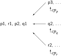
Suppose that we have two processes, p composed of statements p1 followed by p2 and q composed of statements q1 followed by q2, and that the execution is started with the control pointers of the two processes pointing to p1 and q1. Assuming that the statements are assignment statements that do not transfer control, the possible scenarios are:
Note that p2→p1→q1→q2 is not a scenario, because we respect the sequential execution of each individual process, so that p2 cannot be executed before p1.
We will present concurrent programs in a language-independent form, because the concepts are universal, whether they are implemented as operating systems calls, directly in programming languages like Ada or Java,[2] or in a model specification language like Promela. The notation is demonstrated by the following trivial two-process concurrent algorithm:
The program is given a title, followed by declarations of global variables, followed by two columns, one for each of the two processes, which by convention are named process p and process q. Each process may have declarations of local variables, followed by the statements of the process. We use the following convention:
A description of the pseudocode is given in Appendix A.
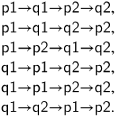
The execution of a concurrent program is defined by states and transitions between states. Let us first look at these concepts in a sequential version of the above algorithm:
At any time during the execution of this program, it must be in a state defined by the value of the control pointer and the values of the three variables. Executing a statement corresponds to making a transition from one state to another. It is clear that this program can be in one of three states: an initial state and two other states obtained by executing the two statements. This is shown in the following diagram, where a node represents a state, arrows represent the transitions, and the initial state is pointed to by the short arrow on the left:
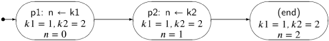
Consider now the trivial concurrent program Algorithm 2.1. There are two processes, so the state must include the control pointers of both processes. Furthermore, in the initial state there is a choice as to which statement to execute, so there are two transitions from the initial state.
The lefthand states correspond to executing p1 followed by q1, while the righthand states correspond to executing q1 followed by p1. Note that the computation can terminate in two different states (with different values of n), depending on the interleaving of the statements.
Example 2.3. Definition
The state of a (concurrent) algorithm is a tuple[3] consisting of one element for each process that is a label from that process, and one element for each global or local variable that is a value whose type is the same as the type of the variable.
The number of possible states—the number of tuples—is quite large, but in an execution of a program, not all possible states can occur. For example, since no values are assigned to the variables k1 and k2 in Algorithm 2.1, no state can occur in which these variables have values that are different from their initial values.
Example 2.5. Definition
A state diagram is a graph defined inductively. The initial state diagram contains a single node labeled with the initial state. If state s1 labels a node in the state diagram, and if there is a transition from s1 to s2, then there is a node labeled s2 in the state diagram and a directed edge from s1 to s2.
For each state, there is only one node labeled with that state.
The set of reachable states is the set of states in a state diagram.
It follows from the definitions that a computation (scenario) of a concurrent program is represented by a directed path through the state diagram starting from the initial state, and that all computations can be so represented. Cycles in the state diagram represent the possibility of infinite computations in a finite graph.
The state diagram for Algorithm 2.1 shows that there are two different scenarios, each of which contains three of the five reachable states.
Before proceeding, you may wish to read the supplementary Section 2.14, which describes the state diagram for an interesting puzzle.
A scenario is defined by a sequence of states. Since diagrams can be hard to draw, especially for large programs, it is convenient to use a tabular representation of scenarios. This is done simply by listing the sequence of states in a table; the columns for the control pointers are labeled with the processes and the columns for the variable values with the variable names. The following table shows the scenario of Algorithm 2.1 corresponding to the lefthand path:
|
|
|
|
|
|
| 0 | 1 | 2 |
|
| 1 | 1 | 2 |
|
| 2 | 1 | 2 |
In a state, there may be more than one statement that can be executed. We use bold font to denote the statement that was executed to get to the state in the following row.
Note
Rows represent states. If the statement executed is an assignment statement, the new value that is assigned to the variable is a component of the next state in the scenario, which is found in the next row.
At first this may be confusing, but you will soon get used to it.
Clearly, it doesn’t make sense to talk of the global state of a computer system, or of coordination between computers at the level of individual instructions. The electrical signals in a computer travel at the speed of light, about 2 × 10⁸ m/sec,[4] and the clock cycles of modern CPUs are at least one gigahertz, so information cannot travel more than 2 × 108 · 10−9 = 0.2 m during a clock cycle of a CPU. There is simply not enough time to coordinate individual instructions of more than one CPU.
Nevertheless, that is precisely the abstraction that we will use! We will assume that we have a “bird’s-eye” view of the global state of the system, and that a statement of one process executes by itself and to completion, before the execution of a statement of another process commences.
It is a convenient fiction to regard the execution of a concurrent program as being carried out by a global entity who at each step selects the process from which the next statement will be executed. The term interleaving comes from this image: just as you might interleave the cards from several decks of playing cards by selecting cards one by one from the decks, so we regard this entity as interleaving statements by selecting them one by one from the processes. The interleaving is arbitrary, that is—with one exception to be discussed in Section 2.7—we do not restrict the choice of the process from which the next statement is taken.
The abstraction defined is highly artificial, so we will spend some time justifying it for various possible computer architectures.
Consider the case of a concurrent program that is being executed by multitasking, that is, by sharing the resources of one computer. Obviously, with a single CPU there is no question of the simultaneous execution of several instructions. The selection of the next instruction to execute is carried out by the CPU and the operating system. Normally, the next instruction is taken from the same process from which the current instruction was executed; occasionally, interrupts from I/O devices or internal timers will cause the execution to be interrupted. A new process called an interrupt handler will be executed, and upon its completion, an operating system function called the scheduler may be invoked to select a new process to execute.
This mechanism is called a context switch. The diagram below shows the memory divided into five segments, one for the operating system code and data, and four for the code and data of the programs that are running concurrently:
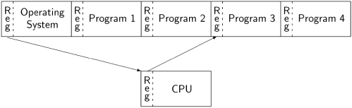
When the execution is interrupted, the registers in the CPU (not only the registers used for computation, but also the control pointer and other registers that point to the memory segment used by the program) are saved into a prespecified area in the program’s memory. Then the register contents required to execute the interrupt handler are loaded into the CPU. At the conclusion of the interrupt processing, the symmetric context switch is performed, storing the interrupt handler registers and loading the registers for the program. The end of interrupt processing is a convenient time to invoke the operating system scheduler, which may decide to perform the context switch with another program, not the one that was interrupted.
In a multitasking system, the non-intuitive aspect of the abstraction is not the interleaving of atomic statements (that actually occurs), but the requirement that any arbitrary interleaving is acceptable. After all, the operating system scheduler may only be called every few milliseconds, so many thousands of instructions will be executed from each process before any instructions are interleaved from another. We defer a discussion of this important point to Section 2.4.
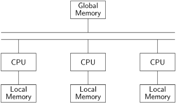
A multiprocessor computer is a computer with more than one CPU. The memory is physically divided into banks of local memory, each of which can be accessed only by one CPU, and global memory, which can be accessed by all CPUs:
If we have a sufficient number of CPUs, we can assign each process to its own CPU. The interleaving assumption no longer corresponds to reality, since each CPU is executing its instructions independently. Nevertheless, the abstraction is useful here.
As long as there is no contention, that is, as long as two CPUs do not attempt to access the same resource (in this case, the global memory), the computations defined by interleaving will be indistinguishable from those of truly parallel execution. With contention, however, there is a potential problem. The memory of a computer is divided into a large number of cells that store data which is read and written by the CPU. Eight-bit cells are called bytes and larger cells are called words, but the size of a cell is not important for our purposes. We want to ask what might happen if two processors try to read or write a cell simultaneously so that the operations overlap. The following diagram indicates the problem:
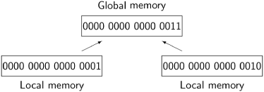
It shows 16-bit cells of local memory associated with two processors; one cell contains the value 0 · · · 01 and one contains 0 · · · 10 = 2. If both processors write to the cell of global memory at the same time, the value might be undefined; for example, it might be the value 0 · · · 11 = 3 obtained by or’ing together the bit representations of 1 and 2.
In practice, this problem does not occur because memory hardware is designed so that (for some size memory cell) one access completes before the other commences. Therefore, we can assume that if two CPUs attempt to read or write the same cell in global memory, the result is the same as if the two instructions were executed in either order. In effect, atomicity and interleaving are performed by the hardware.
Other less restrictive abstractions have been studied; we will give one example of an algorithm that works under the assumption that if a read of a memory cell overlaps a write of the same cell, the read may return an arbitrary value (Section 5.3).
The requirement to allow arbitrary interleaving makes a lot of sense in the case of a multiprocessor; because there is no central scheduler, any computation resulting from interleaving may certainly occur.
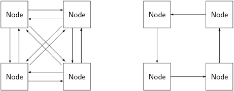
A distributed system is composed of several computers that have no global resources; instead, they are connected by communications channels enabling them to send messages to each other. The language of graph theory is used in discussing distributed systems; each computer is a node and the nodes are connected by (directed) edges. The following diagram shows two possible schemes for interconnecting nodes: on the left, the nodes are fully connected while on the right they are connected in a ring:
In a distributed system, the abstraction of interleaving is, of course, totally false, since it is impossible to coordinate each node in a geographically distributed system. Nevertheless, interleaving is a very useful fiction, because as far as each node is concerned, it only sees discrete events: it is either executing one of its own statements, sending a message or receiving a message.Any interleaving of all the events of all the nodes can be used for reasoning about the system, as long as the interleaving is consistent with the statement sequences of each individual node and with the requirement that a message be sent before it is received.
Distributed systems are considered to be distinct from concurrent systems. In a concurrent system implemented by multitasking or multiprocessing, the global memory is accessible to all processes and each one can access the memory efficiently. In a distributed system, the nodes may be geographically distant from each other, so we cannot assume that each node can send a message directly to all other nodes. In other words, we have to consider the topology or connectedness of the system, and the quality of an algorithm (its simplicity or efficiency) may be dependent on a specific topology. A fully connected topology is extremely efficient in that any node can send a message directly to any other node, but it is extremely expensive, because for n nodes, we need n · (n − 1) ≈n2 communications channels. The ring topology has minimal cost in that any node has only one communications line associated with it, but it is inefficient, because to send a message from one arbitrary node to another we may need to have it relayed through up to n − 2 other nodes.
A further difference between concurrent and distributed systems is that the behavior of systems in the presence of faults is usually studied within distributed systems. In a multitasking system, hardware failure is usually catastrophic since it affects all processes, while a software failure may be relatively innocuous (if the process simply stops working), though it can be catastrophic (if it gets stuck in an infinite loop at high priority). In a distributed system, while failures can be catastrophic for single nodes, it is usually possible to diagnose and work around a faulty node, because messages may be relayed through alternate communication paths. In fact, the success of the Internet can be attributed to the robustness of its protocols when individual nodes or communications channels fail.
We have to justify the use of arbitrary interleavings in the abstraction. What this means, in effect, is that we ignore time in our analysis of concurrent programs. For example, the hardware of our system may be such that an interrupt can occur only once every millisecond. Therefore, we are tempted to assume that several thousand statements are executed from a single process before any statements are executed from another. Instead, we are going to assume that after the execution of any statement, the next statement may come from any process. What is the justification for this abstraction?
The abstraction of arbitrary interleaving makes concurrent programs amenable to formal analysis, and as we shall see, formal analysis is necessary to ensure the correctness of concurrent programs. Arbitrary interleaving ensures that we only have to deal with finite or countable sequences of statements a1, a2, a3,. . ., and need not analyze the actual time intervals between the statements. The only relation between the statements is that ai precedes or follows (or immediately precedes or follows) aj. Remember that we did not specify what the atomic statements are, so you can choose the atomic statements to be as coarse-grained or as fine-grained as you wish. You can initially write an algorithm and prove its correctness under the assumption that each function call is atomic, and then refine the algorithm to assume only that each statement is atomic.
The second reason for using the arbitrary interleaving abstraction is that it enables us to build systems that are robust to modification of their hardware and software. Systems are always being upgraded with faster components and faster algorithms. If the correctness of a concurrent program depended on assumptions about time of execution, every modification to the hardware or software would require that the system be rechecked for correctness (see [62] for an example). For example, suppose that an operating system had been proved correct under the assumption that characters are being typed in at no more than 10 characters per terminal per second. That is a conservative assumption for a human typist, but it would become invalidated if the input were changed to come from a communications channel.
The third reason is that it is difficult, if not impossible, to precisely repeat the execution of a concurrent program. This is certainly true in the case of systems that accept input from humans, but even in a fully automated system, there will always be some jitter, that is some unevenness in the timing of events. A concurrent program cannot be “debugged” in the familiar sense of diagnosing a problem, correcting the source code, recompiling and rerunning the program to check if the bug still exists. Rerunning the program may just cause it to execute a different scenario than the one where the bug occurred. The solution is to develop programming and verification techniques that ensure that a program is correct under all interleavings.
The concurrent programming abstraction has been defined in terms of the interleaving of atomic statements. What this means is that an atomic statement is executed to completion without the possibility of interleaving statements from another process. An important property of atomic statements is that if two are executed “simultaneously,” the result is the same as if they had been executed sequentially (in either order). The inconsistent memory store shown on page 15 will not occur.
It is important to specify the atomic statements precisely, because the correctness of an algorithm depends on this specification. We start with a demonstration of the effect of atomicity on correctness, and then present the specification used in this book.
Recall that in our algorithms, each labeled line represents an atomic statement. Consider the following trivial algorithm:
There are two possible scenarios:
|
|
|
|
| 0 |
|
| 1 |
|
| 2 |
|
|
|
|
| 0 |
|
| 1 |
|
| 2 |
In both scenarios, the final value of the global variable n is 2, and the algorithm is a correct concurrent algorithm with respect to the postcondition n = 2.
Now consider a modification of the algorithm, in which each atomic statement references the global variable n at most once:
There are scenarios of the algorithm that are also correct with respect to the postcondition n = 2:
|
|
|
|
|
|
| 0 |
|
|
|
| 0 | 0 |
|
|
| 1 |
| |
|
| 1 | 1 | |
|
| 2 |
As long as p1 and p2 are executed immediately one after the other, and similarly for q1 and q2, the result will be the same as before, because we are simulating the execution of n←n+1 with two statements. However, other scenarios are possible in which the statements from the two processes are interleaved:
|
|
|
|
|
|
| 0 |
|
|
|
| 0 | 0 |
|
|
| 0 | 0 | 0 |
|
| 1 | 0 | |
|
| 1 |
Clearly, Algorithm 2.4 is not correct with respect to the postcondition n = 2.[5]
We learn from this simple example that the correctness of a concurrent program is relative to the specification of the atomic statements. The convention in the book is that:
Note
Assignment statements are atomic statements, as are evaluations of boolean conditions in control statements.
This assumption is not at all realistic, because computers do not execute source code assignment and control statements; rather, they execute machine-code instructions that are defined at a much lower level. Nevertheless, by the simple expedient of defining local variables as we did above, we can use this simple model to demonstrate the same behaviors of concurrent programs that occur when machine-code instructions are interleaved. The source code programs might look artificial, but the convention spares us the necessity of using machine code during the study of concurrency. For completeness, Section 2.8 provides more detail on the interleaving of machine-code instructions.
In sequential programs, rerunning a program with the same input will always give the same result, so it makes sense to “debug” a program: run and rerun the program with breakpoints until a problem is diagnosed; fix the source code; rerun to check if the output is not correct. In a concurrent program, some scenarios may give the correct output while others do not. You cannot debug a concurrent program in the normal way, because each time you run the program, you will likely get a different scenario. The fact that you obtain the correct answer may just be a fluke of the particular scenario and not the result of fixing a bug.
In concurrent programming, we are interested in problems—like the problem with Algorithm 2.4—that occur as a result of interleaving. Of course, concurrent programs can have ordinary bugs like incorrect bounds of loops or indices of arrays, but these present no difficulties that were not already present in sequential programming. The computations in examples are typically trivial such as incrementing a single variable, and in many cases, we will not even specify the actual computations that are done and simply abstract away their details, leaving just the name of a procedure, such as “critical section.” Do not let this fool you into thinking that concurrent programs are toy programs; we will use these simple programs to develop algorithms and techniques that can be added to otherwise correct programs (of any complexity) to ensure that correctness properties are fulfilled in the presence of interleaving.
For sequential programs, the concept of correctness is so familiar that the formal definition is often neglected. (For reference, the definition is given in Appendix B.) Correctness of (non-terminating) concurrent programs is defined in terms of properties of computations, rather than in terms of computing a functional result. There are two types of correctness properties:
Safety properties. The property must always be true.
Liveness properties. The property must eventually become true.
More precisely, for a safety property P to hold, it must be true that in every state of every computation,P is true. For example, we might require as a safety property of the user interface of an operating system:Always, a mouse cursor is displayed. If we can prove this property, we can be assured that no customer will ever complain that the mouse cursor disappears, no matter what programs are running on the system.
For a liveness property P to hold, it must be true that in every computation there is some state in which P is true. For example, a liveness property of an operating system might be:If you click on a mouse button, eventually the mouse cursor will change shape. This specification allows the system not to respond immediately to the click, but it does ensure that the click will not be ignored indefinitely.
It is very easy to write a program that will satisfy a safety property. For example, the following program for an operating system satisfies the safety property Always, a mouse cursor is displayed:
while true
    display the mouse cursor
I seriously doubt if you would find users for an operating system whose only feature is to display a mouse cursor. Furthermore, safety properties often take the form of Always, something “bad” is not true, and this property is trivially satisfied by an empty program that does nothing at all. The challenge is to write concurrent programs that do useful things—thus satisfying the liveness properties—without violating the safety properties.
Safety and liveness properties are duals of each other. This means that the negation of a safety property is a liveness property and vice versa. Suppose that we want to prove the safety property Always, a mouse cursor is displayed. The negation of this property is a liveness property:Eventually, no mouse cursor will be displayed. The safety property will be true if and only if the liveness property is false. Similarly, the negation of the liveness property If you click on a mouse button, eventually the cursor will change shape, can be expressed as Once a button has been clicked, always, the cursor will not change its shape. The liveness property is true if this safety property is false. One of the forms will be more natural to use in a specification, though the dual form may be easier to prove.
Because correctness of concurrent programs is defined on all scenarios, it is impossible to demonstrate the correctness of a program by testing it. Formal methods have been developed to verify concurrent programs, and these are extensively used in critical systems.
The formalism we use in this book for expressing correctness properties and verifying programs is called linear temporal logic (LTL). LTL expresses properties that must be true at a state in a single (but arbitrary) scenario. Branching temporal logic is an alternate formalism; in these logics, you can express that for a property to be true at state, it must be true in some or all scenarios starting from the state. CTL [24] is a branching temporal logic that is widely used especially in the verification of computer hardware. Model checkers for CTL are SMV and NuSMV. LTL is used in this book both because it is simpler and because it is more appropriate for reasoning about software algorithms.
There is one exception to the requirement that any arbitrary interleaving is a valid execution of a concurrent program. Recall that the concurrent programming abstraction is intended to represent a collection of independent computers whose instructions are interleaved. While we clearly stated that we did not wish to assume anything about the absolute speeds at which the various processors are executing, it does not make sense to assume that statements from any specific process are never selected in the interleaving.
If after constructing a scenario up to the ith state s0, s1,. . ., si, the control pointer of a process p points to a statement pj that is continually enabled, then pj will appear in the scenario as sk for k > i. Assignment and control statements are continually enabled. Later we will encounter statements that may be disabled, as well as other (stronger) forms of fairness.
Consider the following algorithm:
Let us ask the question: does this algorithm necessarily halt? That is, does the algorithm halt for all scenarios? Clearly, the answer is no, because one scenario is p1, p2, p1, p2,. . ., in which p1 and then p2 are always chosen, and q1 is never chosen. Of course this is not what was intended. Process q is continually ready to run because there is no impediment to executing the assignment to flag, so the non-terminating scenario is not fair. If we allow only fair scenarios, then eventually an execution of q1 must be included in every scenario. This causes process q to terminate immediately, and process p to terminate after executing at most two more statements. We will say that under the assumption of weak fairness, the algorithm is correct with respect to the claim that it always terminates.
Algorithm 2.4 may seem artificial, but it a faithful representation of the actual implementation of computer programs. Programs written in a programming language like Ada or Java are compiled into machine code. In some cases, the code is for a specific processor, while in other cases, the code is for a virtual machine like the Java Virtual Machine (JVM). Code for a virtual machine is then interpreted or a further compilation step is used to obtain code for a specific processor. While there are many different computer architectures—both real and virtual—they have much in common and typically fall into one of two categories.
A register machine performs all its computations in a small amount of high-speed memory called registers that are an integral part of the CPU. The source code of the program and the data used by the program are stored in large banks of memory, so that much of the machine code of a program consists of load instructions, which move data from memory to a register, and store instructions, which move data from a register to memory. load and store of a memory cell (byte or word) is atomic.
The following algorithm shows the code that would be obtained by compiling Algorithm 2.3 for a register machine:
The notation add R1,#1 means that the value 1 is added to the contents of register R1, rather than the contents of the memory cell whose address is 1.
The following diagram shows the execution of the three instructions:
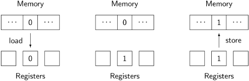
First, the value stored in the memory cell for n is loaded into one of the registers; second, the value is incremented within the register; and third, the value is stored back into the memory cell.
Ostensibly, both processes are using the same register R1, but in fact, each process keeps its own copy of the registers. This is true not only on a multiprocessor or distributed system where each CPU has its own set of registers, but even on a multitasking single-CPU system, as described in Section 2.3. The context switch mechanism enables each process to run within its own context consisting of the current data in the computational registers and other registers such as the control pointer. Thus we can look upon the registers as analogous to the local variables temp in Algorithm 2.4 and a bad scenario exists that is analogous to the bad scenario for that algorithm:
|
|
|
|
|
|
| 0 |
|
|
|
| 0 | 0 |
|
|
| 0 | 0 | 0 |
|
| 0 | 1 | 0 |
|
| 0 | 1 | 1 |
|
| 1 | 1 | |
|
| 1 |
The other type of machine architecture is the stack machine. In this architecture, data is held not in registers but on a stack, and computations are implicitly performed on the top elements of a stack. The atomic instructions include push and pop, as well as instructions that perform arithmetical, logical and control operations on elements of the stack. In the register machine, the instruction add R1,#1 explicitly mentions its operands, while in a stack machine the instruction would simply be written add, and it would add the values in the top two positions in the stack, leaving the result on the top in place of the two operands:
The following diagram shows the execution of these instructions on a stack machine:
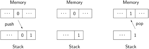
Initially, the value of the memory cell for n is pushed onto the stack, along with the constant 1. Then the two top elements of the stack are added and replaced by one element with the result. Finally (on the right), the result is popped off the stack and stored in the memory cell. Each process has its own stack, so the top of the stack, where the computation takes place, is analogous to a local variable.
It is easier to write code for a stack machine, because all computation takes place in one place, whereas in a register machine with more than one computational register you have to deal with the allocation of registers to the various operands. This is a non-trivial task that is discussed in textbooks on compilation. Furthermore, since different machines have different numbers and types of registers, code for register machines is not portable. On the other hand, operations with registers are extremely fast, whereas if a stack is implemented in main memory access to operands will be much slower.
For these reasons, stack architectures are common in virtual machines where simplicity and portability are most important. When efficiency is needed, code for the virtual machine can be compiled and optimized for a specific real machine. For our purposes the difference is not great, as long as we have the concept of memory that may be either global to all processes or local to a single process. Since global and local variables exist in high-level programming languages, we do not need to discuss machine code at all, as long as we understand that some local variables are being used as surrogates for their machine-language equivalents.
We have specified that source statements like
n ← n + 1
are atomic. As shown in Algorithm 2.6 and Algorithm 2.7, such source statements must be compiled into a sequence of machine language instructions. (On some computers n←n+1 can be compiled into an atomic increment instruction, but this is not true for a general assignment statement.) This increases the number of interleavings and leads to incorrect results that would not occur if the source statement were really executed atomically.
However, we can study concurrency at the level of source statements by decomposing atomic statements into a sequence of simpler source statements. This is what we did in Algorithm 2.4, where the above atomic statement was decomposed into the pair of statements:
temp ← n + 1
n ← temp + 1
The concept of a “simple” source statement can be formally defined:
Example 2.7. Definition
An occurrence of a variable v is defined to be critical reference: (a) if it is assigned to in one process and has an occurrence in another process, or (b) if it has an occurrence in an expression in one process and is assigned to in another.
A program satisfies the limited-critical-reference (LCR) restriction if each statement contains at most one critical reference.
Consider the first occurrence of n in n←n+1. It is assigned to in process p and has (two) occurrences in process q, so it is critical by (a). The second occurrence of n in n←n+1 is critical by (b) because it appears in the expression n+1 in p and is also assigned to in q. Consider now the version of the statements that uses local variables. Again, the occurrences of n are critical, but the occurrences of temp are not. Therefore, the program satisfies the LCR restriction. Concurrent programs that satisfy the LCR restriction yield the same set of behaviors whether the statements are considered atomic or are compiled to a machine architecture with atomic load and store. See [50, Section 2.2] for more details.
The more advanced algorithms in this book do not satisfy the LCR restriction, but can easily be transformed into programs that do satisfy it. The transformed programs may require additional synchronization to prevent incorrect scenarios, but the additions are simple and do not contribute to understanding the concepts of the advanced algorithms.
There are further complications that arise from the compilation of high-level languages into machine code. Consider for example, the following algorithm:
The single statement in process q can be interleaved at any place during the execution of the statements of p. Because of optimization during compilation, the computation in q may not use the most recent value of n. The value of n may be maintained in a register from the assignment in p1 through the computations in p2, p3 and p4, and only actually stored back into n at statement p5. Furthermore, the compiler may re-order p3 and 4 to take advantage of the fact that the value of n+5 needed in p3 is computed in p4.
These optimizations have no semantic effect on sequential programs, but they do in concurrent programs that use global variables, so they can cause programs to be incorrect. Specifying a variable as volatile instructs the compiler to load and store the value of the variable at each use, rather than attempt to optimize away these loads and stores.
Concurrency may also affect computations with multiword variables. A load or store of a full-word variable (32 bits on most computers) is accomplished atomically, but if you need to load or store longer variables (like higher precision numbers), the operation might be carried out non-atomically. A load from another process might be interleaved between storing the lower half and the upper half of a 64-bit variable. If the processor is not able to ensure atomicity for multiword variables, it can be implemented using a synchronization mechanism such as those to be discussed throughout the book. However, these mechanisms can block processes, which may not be acceptable in a real-time system; a non-blocking algorithm for consistent access to multiword variables is presented in Section 13.9.
In Section 2.3, we argued that the proper abstraction for concurrent programs is the arbitrary interleaving of the atomic statements of sequential processes. The main reason why this abstraction is appropriate is that we have no control over the relative rate at which processes execute or over the occurrence of external stimuli that drive reactive programs. For this reason, the normal execution of a program on a computer is not the best way to study concurrency. Later in this section, we discuss the implementation of concurrency in two programming languages, because eventually you will wish to write concurrent programs using the constructs available in real languages, but for studying concurrency there is a better way.
A concurrency simulator is a software tool that interprets a concurrent program under the fine-grained control of the user. Rather than executing or interpreting the program as fast as possible, a concurrency simulator allows the user to control the interleaving at the level of atomic statements. The simulator maintains the data structures required to emulate concurrent execution: separate stacks and registers for each process. After interpreting a single statement of the program, the simulator updates the display of the state of the program, and then optionally halts to enable the user to choose the process from which the next statement will be taken. This fine-grained control is essential if you want to create potentially incorrect scenarios, such as the one shown in Sections 2.5 and 2.8. For this reason, we recommend that you use a concurrency simulator in your initial study of the topic.
This textbook is intended to be used with one of two concurrency simulators: Spin or BACI. The Spin system is described later in Section 4.6 and Appendix D.2. Spin is primarily a professional verification tool called a model checker, but it can also be used as a concurrency simulator. BACI is a concurrency simulator designed as an educational tool and is easier to use than Spin; you may wish to begin your studies using BACI and then move on to Spin as your studies progress. In this section, we will explain how to translate concurrent algorithms into programs for the BACI system.
BACI (Ben-Ari Concurrency Interpreter) consists of a compiler and an interpreter that simulates concurrency. BACI and the user interface jBACI are described in Appendix D.1. We now describe how to write the following algorithm in the dialects of Pascal and C supported by the BACI concurrency simulator:
The algorithm simply increments a global variable twenty times, ten times in each of two processes.
The Pascal version of the counting algorithm is shown in Listing 2.1.[6] The main difference between this program and a normal Pascal program is the cobegin...coend compound statement in line 22. Syntactically, the only statements that may appear within this compound statement are procedure calls. Semantically, upon executing this statement, the procedures named in the calls are initialized as concurrent processes (in addition to the main program which is also considered to be a process). When the coend statement is reached, the processes are allowed to execute concurrently, and the main process is blocked until all of the new processes have terminated. Of course, if one or more processes do not terminate, the main process will be permanently blocked.
The C version of the counting algorithm is shown in Listing 2.2. The compound statement cobegin {} in line 17 is used to create concurrent processes as described above for Pascal. One major difference between the BACI dialect of C and standard C is the use of I/O statements taken from C++.
The BACI dialects support other constructs for implementing concurrent programs, and these will be described in due course. In addition, there are a few minor differences between the standard languages and these dialects that are described in the BACI documentation.
Example 2.1. A Pascal program for the counting algorithm
 1  program count;
 2  var n: integer := 0;
 3  procedure p;
 4  var temp, i : integer;
 5  begin
 6    for i := 1 to 10 do
 7      begin
 8      temp := n;
 9      n := temp + 1
10      end
11  end;
12  procedure q;
13  var temp, i : integer;
14  begin
15    for i := 1 to 10 do
16      begin
17      temp := n;
18      n := temp + 1
19      end
20  end;
21  begin
22    cobegin p; q coend;
23    writeln(' The value of n is ' , n)
24 end.
The Ada programming language was one of the first languages to include support for concurrent programming as part of the standard language definition, rather than as part of a library or operating system. Listing 2.3 shows an Ada program implementing Algorithm 2.9. The Ada term for process is task. A task is declared with a specification and a body, though in this case the specification is empty. Tasks are declared as objects of the task type in the declarative part of a subprogram. It is activated at the subsequent begin of the subprogram body. A subprogram will not terminate until all tasks that it activated terminate. In this program, we wish to print out the final value of the variable N, so we use an inner block (declare . . . begin . . . end) which will not terminate until both tasks P and Q have terminated. When the block terminates, we can print the final value of N. If we did not need to print this value, the task objects could be global and the main program would simply be null; after executing the null statement, the program waits for the task to terminate:
procedure Count is
   task type Count_Task;
   task body Count_Task is. . .end Count_Task;
   P, Q: Count_Task;
begin
   null;
end Count;
Example 2.2. A C program for the counting algorithm
 1  int n = 0;
 2  void p() {
 3    int temp, i;
 4    for (i = 0; i < 10; i ++) {
 5      temp = n;
 6      n = temp + 1;
 7    }
 8  }
 9  void q() {
10    int temp, i;
11    for (i = 0; i < 10; i ++) {
12      temp = n;
13      n = temp + 1;
14    }
15  }
16  void main() {
17    cobegin { p(); q(); }
18    cout << "The value of n is " << n << "
";
19  }
Of course, if you run this program, you will almost certainly get the answer 20, because it is highly unlikely that there will be a context switch from one task to another during the loop. We can artificially introduce context switches by writing the statement delay 0.0 between the two statements in the loop. When I ran this version of the program, it consistently printed 10.
Example 2.3. An Ada program for the counting algorithm
 1  with Ada.Text_IO; use Ada.Text_IO;
 2  procedure Count is
 3     N: Integer := 0;
 4     pragma Volatile(N);
 5     task type Count_Task;
 6     task body Count_Task is
 7        Temp: Integer;
 8     begin
 9        for I in 1..10 loop
10           Temp := N;
11           N := Temp + 1;
12        end loop;
13     end Count_Task;
14  begin
15     declare
16        P, Q: Count_Task;
17     begin
18        null;
19     end;
20     Put_Line("The value of N is " & Integer' Image(N));
21  end Count;
A type or variable can be declared as volatile or atomic (Section 2.9) using pragma Volatile or pragma Atomic:[7]
N: Integer := 0;
pragma Volatile(N);
pragma Volatile_Components and pragma Atomic_Components are used for arrays to ensure that the components of an array are volatile or atomic. An atomic type or variable is also volatile. It is implementation-dependent which types can be atomic.
Example 2.4. A Java program for the counting algorithm
 1  class Count extends Thread {
 2      static volatile int n = 0;
 3      public void run() {
 4        int temp;
 5        for (int i = 0; i < 10; i ++) {
 6          temp = n;
 7          n = temp + 1;
 8        }
 9      }
10      public static void main(String[] args) {
11        Count p = new Count();
12        Count q = new Count();
13        p.start ();
14        q.start ();
15        try {
16          p.join ();
17          q.join ();
18      }
19      catch (InterruptedException e) { }
20      System.out.println ("The value of n is " + n);
21    }
22  }
The Java language has supported concurrency from the very start. However, the concurrency constructs have undergone modification; in particular, several dangerous constructs have been deprecated (dropped from the language). The latest version (1.5) has an extensive library of concurrency constructs java.util.concurrent, designed by a team led by Doug Lea. For more information on this library see the Java documentation and [44]. Lea’s book explains how to integrate concurrency within the framework of object-oriented design and programming—a topic not covered in this book.
The Java language supports concurrency through objects of type Thread. You can write your own classes that extend this type as shown in Listing 2.4. Within a class that extends Thread, you have to define a method called run that contains the code to be run by this process. Once the class has been defined, you can define fields of this type and assign to them objects created by allocators (lines 11–12). However, allocation and construction of a Thread object do not cause the thread to run. You must explicitly call the start method on the object (lines 13–14), which in turn will call the run method.
The global variable n is declared to be static so that we will have one copy that is shared by all of the objects declared to be of this class. The main method of the class is used to allocate and initiate the two processes; we then use the join method to wait for termination of the processes so that we can print out the value of n. Invocations of most thread methods require that you catch (or throw) InterruptedException.
If you run this program, you will almost certainly get the answer 20, because it is highly unlikely that there will be a context switch from one task to another during the loop. You can artificially introduce context switches between between the two assignment statements of the loop: static method Thread.yield () causes the currently executing thread to temporarily cease execution, thus allowing other threads to execute.
Since Java does not have multiple inheritance, it is usually not a good idea to extend the class Thread as this will prevent extending any other class. Instead, any class can contain a thread by implementing the interface Runnable:
class Count extends JFrame implements Runnable {
   public void run() { . . . }
}
Threads are created from Runnable objects as follows:
Count count = new Count();
Thread t1 = new Thread(count);
or simply:
Thread t1 = new Thread(new Count());
A variable can be declared as volatile (Section 2.9):
volatile int n = 0;Variables of primitive types except long and double are atomic, and long and double are also atomic if they are declared to be volatile. A reference variable is atomic, but that does not mean that the object pointed to is atomic. Similarly, if a reference variable is declared as volatile it does not follow that the object pointed to is volatile. Arrays can be declared as volatile, but not components of an array.
Example 2.5. A Promela program for the counting algorithm
 1  #include "for.h"
 2  #define TIMES 10
 3  byte  n = 0;
 4  proctype P() {
 5     byte temp;
 6     for (i ,1, TIMES)
 7         temp = n;
 8         n = temp + 1
 9     rof (i)
10  }
11  init {
12      atomic {
13         run P();
14         run P()
15      }
16      (_nr_pr == 1);
17      printf ("MSC: The value is %d
", n)
18  }
Promela is the model specification language of the model checker Spin, which will be described in Chapter 4. Here we describe enough of the syntax and semantics of the Promela language to write a program for Algorithm 2.9.
The syntax and semantics of declarations and expressions are similar to those of C, but the control structures might be unfamiliar, because they use the syntax and semantics of guarded commands, which is a notation commonly used in theoretical computer science. A Promela program for the counting algorithm is shown in Listing 2.5, where we have used macros defined in the file for.h to write a familiar for-loop.
The process type P is declared using the keyword proctype; this only declares a type so (anonymous) instances of the type must be activated using run P(). If you declare a process with the reserved name init, it is the first process that is run.
Promela does not have a construct similar to cobegin, but we can simulate it using other statements, run and atomic. The run P() statements activate the two processes. atomic is used to ensure that both activations are completed before the new processes begin; this prevents meaningless scenarios where one or more processes are never executed.
The join (waiting for both processes to finish before continuing) is simulated by waiting for _nr_pr to have the value 1; this is a predefined variable counting the number of active processes (including init).
When the two processes have terminated, the final value of n is printed. The prefix MSC is a convention that is used by postprocessors to display the output of the program.
This section demonstrates state diagrams using an interesting puzzle. Consider a system consisting of 2n+1 stones set in a row in a swamp. On the leftmost n stones are male frogs who face right and on the rightmost n stones are female frogs who face left; the middle stone is empty:
Frogs may move in the direction they are facing: jumping to the adjacent stone if it is empty, or if not, jumping over the frog to the second adjacent stone if that stone is empty. For example, the following configuration will result, if the female frog on the seventh stone jumps over the frog on the sixth stone, landing on the fifth stone:
Let us now ask if there is a sequence of moves that will exchange the positions of the male and female frogs:
This puzzle faithfully represents a concurrent program under the model of interleaving of atomic operations. There are 2n processes, and one or more of them may be able to make a move at any time, although only one of the possible moves is selected. The configuration of the frogs on the stones represents a state, and the transitions are the allowable moves.
It is easy to put an upper bound on the number of possible states: there are 2n frogs and one empty place that can be placed one after another giving (2n + 1)!/(n! .n!) possible states. The divisor n! ·n! comes from the fact that all the male frogs and all the female frogs are identical, so permutations among frogs of the same gender result in identical states. For n = 2, there are 30 states, and for n = 3, there are 140 states. However, not all states will be reachable in an actual computation.
To build a state diagram, start with the initial state and for each possible move draw the new state; if the new state already exists, draw an arrow to the existing state. For n = 2, Figure 2.1 shows all possible states that can occur if the computation starts with a move by a male frog. Note that the state ⨿ MMFF can be reached in either one or two moves, and that from this state no further moves are possible as indicated by the symbol ×.
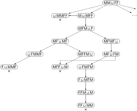
From the diagram we can read off interesting correctness assertions. For example, there is a computation leading to the target state FF ⨿ MM; no computation from state MF ⨿ MF leads to the target state; all computations terminate (trivial, but still nice to know).
This chapter has presented and justified the concurrent program abstraction as the interleaved execution of atomic statements. The specification of atomic statements is a basic task in the definition of a concurrent system; they can be machine instructions or higher-order statements that are executed atomically. We have also shown how concurrent programs can be written and executed using a concurrency simulator (Pascal and C in BACI), a programming language (Ada and Java) or simulated with a model checker (Promela in Spin). But we have not actually solved any problems in concurrent programming. The next three chapters will focus on the critical section problem, which is the most basic and important problem to be solved in concurrent programming.
1. | How many computations are there for Algorithm 2.7. | |||||||||
2. | Construct a scenario for Algorithm 2.9 in which the final value of | |||||||||
3. | (Ben-Ari and Burns [10]) Construct a scenario for Algorithm 2.9 in which the final value of | |||||||||
4. | For positive values of | |||||||||
5. | (Apt and Olderog [3]) Assume that for the function f, there is some integer value i for which f (i) = 0. Here are five concurrent algorithms that search for i. An algorithm is correct if for all scenarios,both processes terminate after one of them has found the zero. For each algorithm, show that it is correct or find a scenario that is a counterexample. In process Table 2.15. Zero E
| |||||||||
6. | Consider the following algorithm where each of ten processes executes the statements with
| |||||||||
7. | Consider the following algorithm:
| |||||||||
8. | Consider the following algorithm:
| |||||||||
9. | Consider the following algorithm:
| |||||||||
10. | Consider the following algorithm:
| |||||||||
11. | Complete Figure 2.1 with all possible states that can occur if the computation starts with a move by a female frog. Make sure not to create duplicate states. | |||||||||
12. | (The welfare crook problem, Feijen [3, Section 7.5]) Let
| |||||||||
[1] Alternate terms for this concept are instruction pointer and location counter.
[2] The word Java will be used as an abbreviation for the Java programming language.
[3] The word tuple is a generalization of the sequence pair, triple, quadruple, etc. It means an ordered sequence of values of any fixed length.
[4] The speed of light in a metal like copper is much less than it is in a vacuum.
[5] Unexpected results that are caused by interleaving are sometimes called race conditions.
[6] By convention, to execute a loop n times, indices in Pascal and Ada range from 1 to n, while indices in C and Java range from 0 to n − 1.
[7] These constructs are described in the Systems Programming Annex (C.6) of the Ada Language Reference Manual.