CHAPTER 6

The Source of Value

To this point in the book, I’ve talked a lot about this notion of cash value. One important question is, “What is cash value?” This chapter will delve into answering this question by creating a contextual definition of value, discussing where value comes from in the context of improvement projects, and then discussing the path to cash value via capacity improvements. I will do this by focusing on answering the following questions:

What Is Value?

We often hear people using the term value freely and ambiguously. The question is, “What is value?” I believe it is important that we define the term so that we can eliminate as much ambiguity as possible. This will put us all on the same page and allow us to understand and work toward common goals.

Value, here, is defined simply as the positive effect created by the improvement project. More specifically, think about answering the following questions:

“What will be better as a result of implementing this project?”

“Why will it be better?”; and

“To what extent?”

These elements will help us understand, define, and document how the project will improve the business. Additionally, since this book is focused on cash generation, we will understand whether the improvement itself can lead to cash improvement, and if not, help us define the steps that are necessary to achieve the cash value. This process begins with documenting the direct value the improvement project has.

Documenting Value

For us to see the impact or anticipated impact from the project, we have to document the changes that are directly created by the project. If we go back to Chapter 4, the Operations and Cash, or OC Domain was central to modeling operations, cash, capacity, and business activity. Recall, also, the four key business activities of the BCC Model buy, consume, create, and sell.

Capacity maps, as discussed in Chapter 4, are an effective tool for modeling the OC Domain and the associated business activities. As mentioned previously, capacity maps help us understand how much capacity we’ve bought and what the cash implication is, how much we’ve consumed, how much output was created, and of that, how much was sold (Figure 6.1). For example, looking at Figure 6.2, we see if we pay $30 per hour for the capacity, we know we bought eight hours for $240. We know we consumed seven of the eight hours or 87.5 percent of the capacity we bought and created 56 units of output for an average of eight units per productive hour or seven units per purchased hour. Adding sales, assuming we sell 50 of them for six dollars each, we would generate $300 in revenue this period assuming all sales are recovered in the current period (Figure 6.3). Hence, we have generated $300 and spent $240 for the period suggesting we made $60 cash. We know this without calculating a single unit cost. We can also see we produced in excess of demand suggesting we were overproductive.

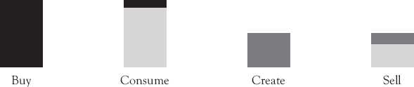
Figure 6.1 Capacity maps represent how business is transacted, from buying capacity, through consuming that capacity to create output. When the output is salable, it compares how much output was created to the demand for the output. From capacity maps comes a wealth of information on cash, business activity, and business efficiency, effectiveness, and efficacy

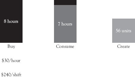
Figure 6.2 This is a traditional capacity map without sales being shown. It describes how much capacity we bought, what we paid for it, how much of the capacity was consumed, and how much output was created from the consumed capacity

For the purposes of this book, and as suggested generally when using the Business Domain Management framework, we will focus on modeling business and cash activities in the OC Domain using capacity maps.¹ This is where the business activity happens and will be the target for improvement projects. It is where we make decisions regarding how much capacity we need, when we buy it, how much we buy, and how we will use it. This affects cash_OUT. It’s also where we make the decisions regarding output levels, which influences our efficiency, effectiveness, and productivity. Finally, it’s where we actually create output, whether for external or market purchase and consumption, or used internally by coworkers. This helps us understand the demand for capacity. When we understand capacity and capacity consumption rates, we can start with demand, determine how much capacity is necessary to meet that demand at both current and post improvement rates, and then back into the amount of capacity we need to buy, which is critical when managing cash_OUT.

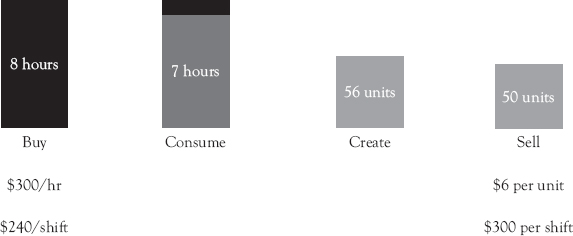
Figure 6.3 Here, we have a capacity map that considers both sales and demand. Demand for output, whether salable or not, should set the context for how much capacity we need and to buy, how we consume it, and how much output it should create. For instance, in this case, we see that we created more output than was necessary, suggesting we could potentially meet demand with less capacity. Notice we did not have this context in Figure 6.2

When output is salable, it may help our cash_IN. In Figure 6.3, we can see that we exceeded demand, so although there were more items to sell, if there is no demand, there are no sales. This challenges the notion that generally increasing output will lead to sales. This is not true as discussed in Chapter 2.

These elements of the business are exactly what improvement projects focus on, and where they will subsequently create value. For instance, in Figure 6.4, we can see that we have created value by reducing the amount of input necessary to create the same level of output. By documenting how we do business initially and how things would be in the future as a result of the improvement project using capacity maps, we should see discernible differences between the two.

Figure 6.4 This capacity map shows how many techniques create value. By requiring less capacity to create output, companies now have additional capacity that can either be filled with value adding work or eliminated if not needed. Because the amount of capacity we buy has not changed in this case, the improvement will not affect cash_OUT

Types of Value

There are two types of value that improvement projects create and that we will focus on. The first is the operational value described previously. This is the improvement to operations that can or will result from implementing the project. The second is the marginal improvement in cash resulting from or enabled by the project.

The path to cash value (Figure 6.5) will begin by creating operational value. How will operations be improved as a result of our project, as shown with capacity maps. However, this is not enough. The reason is, improvement projects improve our efficiency in the context of creating output. As we will see later in the chapter, cash is spent on what we buy, so even if we can create more output or take less capacity to create output, if the amount we buy does not change, there will be no cash savings. In many cases, additional managerial steps must be executed to achieve the cash value. For instance, looking at Figure 6.4, we can see that the same amount of money was spent before the improvement as we spent after the improvement.

Figure 6.5 The path to value realization involves improving the current state (As-Is) to a future state (To-Be). The To-Be state should enable an improvement to the As-Is state. However, the changes do not usually happen automatically. Oftentimes, managerial action will be required to achieve the operational value

Likewise, with sales limited to 50 units in the example, revenue will be capped at $300. The improvement had no cash benefit as demonstrated by the capacity map. Only when we make changes will we see changes in cash. If we take managerial steps, we can realize cash savings as demonstrated shown in Figure 6.6. Initially, we since we can create the same output with less input, we can buy less input and still be as productive.

Figure 6.6 The operational value in this case is tied to reducing capacity consumption from 7 to 6 hours. In A, we have the current state situation. In B, we can see that the same level of output can be created with fewer hours. This allows us to reduce the amount of capacity purchased (from 8 to 7, reducing cash_OUT by $30. In C, by aligning output, we reduce the amount of capacity necessary to meet demand. This allows for a further reduction in capacity of one hour. Notice, however, that capacity costs are only saved when management buys less capacity

If we look to align output with demand, we will find an even greater opportunity to reduce cash_OUT. We can actually meet demand by buying six hours of capacity rather than eight, saving $60 in the process. This doesn’t happen automatically, however. Someone must purposefully change how much capacity is purchased for the cash savings to be realized. Repurposing people is positive from a human resources perspective, but it will have no effect on cash_OUT. There will be more on this in Chapter 7.

How Do Improvement Projects Create Value?

To understand how improvement projects create value, we need to first consider what will be improved. Let’s begin by taking a deeper dive into capacity. We buy capacity in the form of labor, space, materials, equipment, and technology. When we buy this capacity, the following is usually the case; we pay an amount for a fixed amount of capacity and the cash cost does not change with use. For instance, what we pay for 5,000 square feet does not change with how we use it, just like your salary does not change with the work that you do. Likewise, what we pay for materials doesn’t change when we consume it. It only changes with what we buy. This type of capacity is called static or input capacity. It is static because we buy a fixed amount. It is input because it’s what we will start with to create output. Without this capacity, we would not be able to create output. We would need to rely on another source.

The second type of capacity is dynamic or output capacity. Output capacity is what we can create with the input capacity. Offices and storage space as outputs are made available from the space input we bought. Widgets as output are created from the labor, material, and equipment capacity we bought. Projects, as output, are created, executed, and delivered from the labor capacity we bought.

Because output can vary, it is dynamic and referred to as dynamic capacity.² Two people may, based on differing skill sets, have different output levels when doing the same work over the same period. The same person will have varying output levels for the same amount of time at different moments. For instance, our productivity in the morning for one hour may be different from our productivity during an hour in the afternoon.

There is a theoretical maximum output level and the actual realized output level.³ Both play a role in capacity planning and management. Theoretical helps us understand what is truly possible while the actual helps us understand what we achieved. The two do not need to be the same. In fact, as we will see later in the chapter, the actual should be tied to creating an efficient, effective, and productive way to meet demand when looking to focus on cash. We will see that accounting information may sometimes drive us, unnecessarily, toward aligning them, which may suboptimize overall performance.

Improvement projects create operational value by increasing efficiency. Efficiency is defined as the ratio of output to input (Equation 6.1).

Efficiency as an expression of capacity is found in Equation 6.2.

We are familiar with this relationship. Consider fuel efficiency. We buy one gallon of gas (input), and we drive (output). Assuming we go 20 miles and use the entire gallon of gas, we will say that our fuel efficiency is 20 miles per gallon. Now assume either improvements in driving style, conditions, or improvements to the vehicle now allow you to drive 25 miles on a gallon of gas. You have increased your fuel efficiency from 20 miles per gallon to 25 miles per gallon (Figure 6.7). With this improvement, you can either drive farther with the same input, or go the same distance with less input.

The same holds true with our work. Assume there are 10 customer service issues to be addressed by 5 customer service reps. If we can automate the process so that only four reps are required, we have increased our efficiency.

Improvement projects generally target efficiency improvements in general, and improvements to consumption, and output rates specifically. When you consider the benefits of IT, for example, you may get data and information faster, it may be of higher quality, or its value to you is now much greater. You can get the same work done in less time. These examples are like driving 20 miles using less gas. When you reach the desired destination, you’d have more input capacity, gas, than you normally would. You can get to your desired output level using less capacity because your IT solution has simplified tasks, for example. The other side of IT improvements is that they may allow you to get more accomplished in the same amount of time. This is akin to being able to drive farther with one gallon. In the same period, you can process more invoices or sign off on more documents.

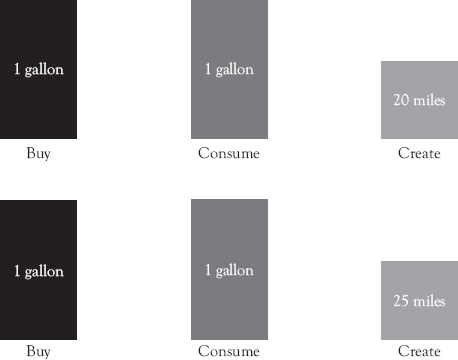
Figure 6.7 This capacity map shows creating more output with the same input increases efficiency. For the same investment in input, we can get greater output. This is one example of an efficiency increase. Another example comes from considering there is less capacity required to meet demand. For example, if you only need to go 20 miles, you no longer need a full gallon of gas. You only need 8/10 of a gallon of gas. Hence, you can create the same output using less input

In the end, you are more efficient, but that you are more efficient doesn’t mean your company is paying less for capacity. They are not paying you less. They’re paying you the same, so cash_OUT remains exactly the same and in this context, forgetting about the investment to realize the improvement, the cash level stays the same. This is where I encounter resistance from naysayers discussing what else they believe the improvements enable:

What we see is that to reduce cash costs, cost_C, we must change input capacity. We either buy less or we buy cheaper. Improvements can only affect output capacity. Input capacity changes with managerial decisions that are enabled by, not because of, the improvements. Improvement projects don’t cause changes in how much input capacity is purchased as much as gravity doesn’t cause plane crashes. Something must change that enables other factors to take over.

Going back to Figure 6.6, the improvements enabled managers to choose whether they reduced capacity to save on cash_OUT. They can choose to continue to buy eight hours for no savings, or they can buy seven or six, but these are managerial decisions that must be made and executed.

How Do We Manage Cash Value Realization?

Efficiency brings us operation value. However, we are seeking cash value which, I hope I’ve demonstrated, doesn’t come directly from efficiency improvements. We need the appropriate management actions to convert the operational value to cash value. This happens when we execute decisions that affect cash_IN and cash_OUT. This is very important. Managers who do not understand the nature and impact of the improvement and, therefore, what actions they should take can have a neutral value on cash at best and negative value at worst.

Figure 6.8 When the amount of cash remains the same, there have been no cash benefits. Cost per unit is an Accounting Domain metric that creates an illusion that costs are decreasing. Can you name one scenario where you spend less money making 20 of something than you would making just two?

Consider the following example of how managers can be bamboozled by an inappropriate understanding of, or approaches to improving cash. In Figure 6.9, we have three step or three operation process to create salable output. The maximum output of this process is five units per hour as constrained by Operation 2. A consultant comes along and demonstrates how Operation 1’s efficiency can be increased by 20 percent from 10 units per hour to 12 units per hour (Figure 6.10). Generally, this would create an accounting cost savings but as we can see from the capacity map in Figure 6.11, there has been no change in cash.

What we have here can be easily explained using what I call an isocash curve. As a prefix, iso means same or equal. Isocash, therefore, means same or equal cash. What we pay the person for the shift in this case is $30 per hour as shown in Figure 6.12.

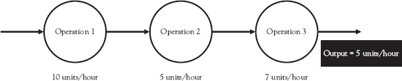
Figure 6.9 A simple three-step process helps us understand the impact of constraints on processes

Figure 6.10 Notice that we have increased the output rate of Operation 1, but the output rate of the process has not changed. This means both the output and the revenue (assuming there is demand, that is ≥ 5 units per hour) are constrained by Operation 2. Improving A will have no direct positive cash improvement, and considering the company may have paid for the improvement and the excess materials to take advantage of the increase, there may be a negative cash impact

Figure 6.11 This is a capacity map for Operation 1. As we can see, nothing changes from a cash_OUT perspective in the OC Domain even though we can calculate a cost savings for the improvement in the Accounting Domain

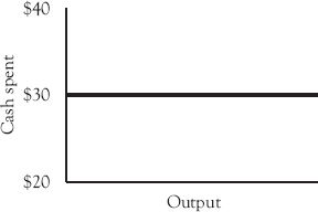
Figure 6.12 The $30 spent for an hour of Operation 1 and the output created are independent of one another

This curve, as we have seen several times before, shows the relationship between what we paid for the capacity and the output created by it. They are, of course, independent. However, when we tried to transform OC Domain data into accounting information, something strange happens. In Figure 6.13, what we see is an isocash curve for one hour of the person’s time. In that one hour, we see that as we increase output, we get the impression that unit costs are going down. In this example, we pay the person $30 per hour. If we divide this by units of output, we have one way to calculate a unit cost. Initially, we spent $30 and created 10 units for a cost of three dollars per unit. By increasing the output to 12, we see the cost is reduced to $2.50. From this curve, we see that as we create more output, the cost per unit goes down. However, this is cost_NC.

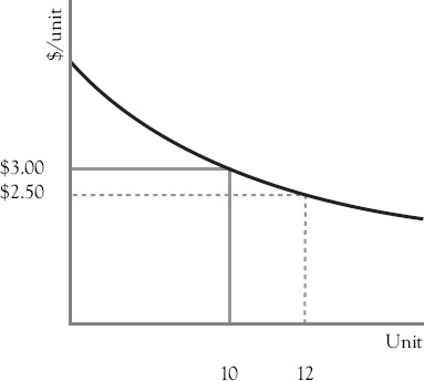
Figure 6.13 This is a typical isocash curve. It is isocash because the curve represents one value of cash. In this case, the cash represents the $30 for an hour of labor. Cost per unit can be calculated from the curve as we see in this case. The curve shows that the cost per unit goes down with increased output although cash spent remains the same

This leads to an extremely important conclusion. Most people in their right mind may consider improving Operation 1 and lowering its unit cost to be a positive. However, the cash_OUT is the same or higher. Assume we spent money on the solution. Our cash_OUT has increased due to the services purchased and received. To get full value from the improvement, one may want maximum use of the capacity. The more products created, the lower the accounting cost. So, the company increases its material consumption rate and therefore the rate of buying material capacity. Seeking efficiency in this case may lead to higher input costs to achieve the artificial $0.50 savings per unit. Additionally, assuming no increase in sales but recognizing the unit cost reduction, selling the product at a higher gross margin can lead to a higher tax base. Given the revenue is five dollars for an initial margin of two dollars versus $2.50 after the improvement, with a higher gross margin, we are increasing our taxable income, which increases cash_OUT.

This analysis does two things. First, it demonstrates what happens when people focus on accounting value rather than cash value. Decisions can be made in the name of reducing costs or improving profit that have no, or a negative effect on cash. Second, it will discourage actions and decisions that appear positive financially but can be to the company’s detriment. Here are a few examples of both.

I once visited a company that made corrugated paper products. During the plant tour, the plant manager bragged about a huge piece of equipment called a corrugator. He mentioned how expensive it was to buy, and to “pay back” the machine, they needed to run it all the time. The facility was in a small town, and the plant manager mentioned that the machine supported the local economy. Why was it felt that the corrugator must be running all the time to “pay for itself” and to “reduce costs?”

Keeping the corrugator running 24/7, for instance, required a lot of labor, material, equipment and space capacity to feed it, run it, unload it, and to store the final product. Later in the tour, we visited the finished goods area where there was inventory everywhere and most had no customer orders tied to it.

One must ask how running a machine and building inventory that is not sold saves money. How does it “pay back” the machine? If more labor and materials are purchased, cash_OUT is increasing, yet with finished goods sitting in inventory, there is not a subsequent increase in sales, suggesting that the company is worse off financially not better. So why does this happen?

The primary reason there is focus on efficiency is because of how the improvements are handled in the Accounting Domain. We believe that by increasing efficiency, our costs go down as demonstrated in the isocash curve in Figure 6.13. Recall the two ways of increasing efficiency. The first is to create more output with the same input. The second is to reduce the amount of capacity consumed to create current levels of output as seen in the isocash curve shown in Figure 6.14. In both cases, we see a reduction in the Accounting Domain metric of cost per unit without a subsequent change to cash_OUT. This causes many to believe they are improving the situation financially when, in fact, they are doing little at best, and damage at worst. By running the corrugator 24/7, the plant manager was extending the “payback” not shortening it, and spending money, not making it.

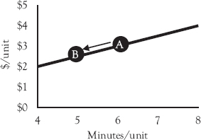
Figure 6.14 This is an example of an isocash curve that considers consumption rates versus output. It represents reductions in cost per unit related to reductions in consumption rates

The second scenario was one I experienced as a professor. In a course designed for graduating seniors, the professor created a problem that compared having an older piece of equipment to a newer piece of equipment and asked the students to compare the scenarios as somewhat of an improvement project. The professor mentioned the salvage value of the older equipment, the price of the newer equipment, improvements in output rates, depreciation rates, and so on. Many of us have performed these analyses.

Nowhere did the professor mention whether the machine was going to improve a nonconstraint such as Operation 1 or whether it was going to be applied to a constraint such as Operation 2, which would improve process output. When performing the financial analysis as set up by the professor, the company in question might spend $40 million on a piece of equipment that would potentially have no effect on cash_IN. There would be, however, a significant increase in cash_OUT, which could leave the company in a much poorer position.

Managers are still learning these techniques in universities and by others in their companies, and it leads to poorer, not better, cash performance from improvement projects. If we want improvements to cash, we must model cash and make decisions that affect cash_IN and cash_OUT.

Focusing on Accounting Domain information rather than OC Domain cash data will practically guarantee that managerial decision making will suboptimize and, in some cases, sabotage cash value.

Next chapter, we will focus on how to design improvements that do focus on cash and lead us toward the cash improvement we seek.

Key Takeaways

¹ Lee 2018.

² Ibid, 58.

³ R.T. Yu-Lee. 2003. “Don’t Miss the Bottom Line with Productivity.” Increases Industrial Management, 8–13.