CHAPTER 8

Financial Benefits and Benefit Projection

Thus far in the book, we’ve focused on getting to the point where we can design our improvements to realize cash value. We started by focusing on what it takes to realize cash benefits. We then looked at the types of improvement projects there are, how they generate value, the steps necessary to document the improvements, and the management action required to realize cash improvements. This chapter is focused on documenting the benefits and projecting them into the future so that we know when to expect cash benefits and how much to expect.

Key to this process will be using the BCC Model and the capacity maps we created in Chapter 7. As we have seen, capacity maps are used to describe the input capacity levels, capacity consumption rates, and output rates. Since this chapter is focused on identifying the financial value of the improvement, capacity maps will show, clearly, where there are and are not cash benefits. This is where people would typically use cost, managerial accounting, or cost accounting information. However, as discussed in Chapters 3 and 4, accounting information is not useful when calculating the cash benefits and profitability of a project. In fact, it can sometimes be harmful.

Recall, cost and managerial accounting create cost values that are not cash. For instance, consider the following scenario discussed in Chapter 6. We started with an As-Is capacity map where we buy an hour of time for $30. The current output level is 10 units. One possible cost would be $3 per unit when using the entire hour as a cost basis (Figure 8.1).

After the improvement, we assumed output increased from 10 to 12 with the same capacity consumption rates (Figure 8.2). There may be a calculated cost reduction of 50 cents as shown in Figure 8.3. However, we are still on the same isocash curve suggesting nothing has changed from a cash perspective. Hence, the direct cash savings opportunity is zero. The harm comes from assuming these cost savings represent cash and, therefore, are used in the financial justification of the project. They do not represent cash and should not be used to justify projects on a cash basis. This doesn’t mean there is no benefit opportunity, as there are noncash opportunities that result from the improved use of capacity. As discussed several times previously, the initial lack of cash savings doesn’t mean there is no opportunity for cash improvement. The improved use of capacity may enable managerial decisions, and it’s the management action that creates the cash improvement. It is here where we should focus our cash value creation efforts. When calculating the improvements in cash, we want to focus specifically on factors that affect cash_IN and cash_OUT, as these are the only factors that affect cash (Figure 7.5). Let’s discuss both.

Figure 8.1 Our initial capacity map before improvements are made to output

Figure 8.2 With an increase in output rate with the same buy– consume attributes, we can calculate a lower unit cost even though the cash_OUT has not changed

Figure 8.3 This isocash curve shows why there is no change in cash_OUT from the capacity map in Figure 8.2

Cash_IN

The focus with cash_IN is documenting the extent to which there will be an improvement in the rate and timing of cash coming into the organization. There can be a significant difference between the two, so understanding this difference is key. In one case, the issue is about creating a marginal increase in cash_IN, such as when there is an increase in sales. From increased sales, cash_IN may increase from $1,000 per day, for instance, to $1,200, and this increase is solely from increasing the daily sales rate. The other situation is about timing of accounts receivable. If sales are $1,000 per day but day sales outstanding is 45 days, there may be opportunities to collect the cash in fewer days. While improving collections, there may be an increase in daily cash receipts, but that is only collecting what is already due in, so there is no increase in sales. Hence, while there may be increases in cash receipts initially, once outstanding receivables get down to the target levels, the cash_IN rate will will be represented by a delay in the rate of sales.

In the first case, the challenge is determining the extent to which revenue will be increased. To increase sales, the improvement project must lead to increased demand and there must be the ability to meet it, either currently or by increasing the output levels. With this, there is a level of uncertainty involved with estimating the increase in sales because demand is often not known with certainty. What is the growth potential? We hope, at a minimum, we will maintain our current sales after the improvement project, but what will the maximum be? If the improvement project increases output potential, how much of the increased output will be absorbed by the market?

In cases like this, as mentioned in the last chapter, we will want to bound the opportunity to help deal with the uncertainty. Ideally, the future sales will not dip below current sales. However, through solution design and bounding the projections, we will need to carefully document what could happen, or not, that may cause a reduction in sales. If there is enough knowledge of an increase in demand, the lower bound may be higher than our current sales. On the high end, there will have to be a guess, and this value is tied to how you handle uncertainty. The higher the uncertainty, the greater the risk, so managing the uncertainty is key to effective projections.

When there is uncertainty, it is tied to that which is unknown (Figure 8.4). ¹ All that is initially unknown is not unknowable, however. Market research, for instance, which may range from surveys to asking for sales commitments, may help you understand some element of the unknown potential demand. The objective is to work to minimize the unknown (Figure 8.5). The upper and lower bounds on the improvement continuum will become closer in value as uncertainty is reduced.

Figure 8.4 In the world of information, there is that which is known and that which is unknown

Figure 8.5 How much of that which is currently unknown is truly unknowable? The unknown drives uncertainty and, therefore, risk. If we can reduce that which is unknown but not unknowable, we can reduce uncertainty

The keys to improving cash through increasing sales are, (1) State the assumptions for the boundaries by asking what must be true for the optimistic projections to be realized, and what must go wrong for the pessimistic assumptions to come true so we understand what is required to achieve the benefits we seek, and (2) manage overactivity in the name of being overly optimistic. Overactivity in this context means buying more than is necessary or creating more than is necessary. There is a risk to optimism, as it can lead to a negative impact on cash when wrong. Oftentimes, extra capacity is purchased in anticipation of creating excess salable output. The money is spent, the output is created, and the sales do not come as anticipated or desired.

The capacity impact of overproduction is often hidden by the numbers in the Accounting Domain. For instance, excess inventory is put on the balance sheet, and as a result, the impact of the decision, from a cash perspective, is difficult to see. Can you see the cash impact of overtime, used to create excess output, on the next payroll cycle clearly by looking at inventory on the balance sheet? The answer is, “no.” In fact, the increased output may even lower the product cost, leading to a potential incentive to create more output, all without knowing or realizing the negative impact of the increased cash_OUT.

In estimating sales increases, in addition to bounding the amount of the increase, we will have to consider the timing. When considering increased output, we will have to think about the particulars regarding how output will be increased, the steps to implement these particulars, and then the expected rate and timing of increase of sales. These are important when determining how long it will take to realize the increased cash_IN, compared to the expenditures necessary to realize the value.

Regarding the timing of cash receipts, there are a couple factors to consider.

Having the Cash Creates

There are many benefits associated with having cash from reducing receivables, such as less time and, therefore, capacity involved in collecting it, and the ability to invest the capital for longer periods. The key will be to model the improvements and management actions effectively. If there were capacity used collecting cash, how much of that capacity can be freed by reducing the demand on it from the collections activities? What will this enable management to do to affect cash_OUT? It’s quite possible it won’t, but the opportunity should be considered. If the capacity is not reduced, cash_OUT will not change. Additionally, improved working capital investment requires the cash to actually be invested; sooner rather than later. If you have the cash and do not make it work for you, the ability for it to generate more cash is compromised. We will want to model the cash_OUT for the investment and any returns we may anticipate, but only those we anticipate during the analysis period. Clearly, with investments, we are dealing with uncertainty based on the type of investments and the variability/risk involved, so both the benefit and the timing of the return will need to be bounded.

What Having the Cash Eliminates

Having the cash does two things. First, as mentioned previously, there is less of a need to chase the cash, so less capacity will be spent doing so, and resorting to actions such as factoring the receivables, which can lead to a lower cash_IN and the potential for an increased cash_OUT to cover the costs of factoring can be avoided. A second key concept is that by having the money, hopefully the need for future loans can be reduced. Clearly this reduces the cash impact of borrowing the money.

The keys with cash_IN are to be diligent in modeling the improvement, the steps or managerial actions necessary to achieve the benefits, and to state the assumptions when bounding the opportunities. Oftentimes, the optimism is too high and the pessimism is too low because of the pressure to show improvement. It’s best that both are tempered, challenged, and the assumptions stated and agreed on so that the projections are believed to be more realistic.

Cash_OUT

The largest opportunities are generally found by adjusting cash_OUT. As mentioned several times throughout the book, improvements are enabled by making capacity more efficient. We also learned efficiency improvements keep you on the same isocash curve and, therefore, do not lead to reductions in cash_OUT. To achieve the benefits in cash_OUT, you must move to another isocash curve (Figure 8.6). This happens when you change the amount of input capacity you buy or the price you pay for it. These changes lead directly to cash improvements. The difference between the input capacity levels on the As-Is capacity map and the To-Be capacity map becomes the source of documenting the cash value opportunity. How much less capacity at a given price are we buying? How much of the same capacity at a lower price are we buying? The management action involves the steps necessary to shift operations from the current state to the desired state. This process simply involves documenting the cash value of the capacity reduction created by management action.

Figure 8.6 Increasing efficiency by going from A to B will lower the unit cost. However, it will not affect cash_OUT. Moving from A to A’ is a shift in isocash curves, repesenting a lower cash_OUT

As we look to document the cash benefit of the changes, we have to be diligent and precise about what has changed. When we think about capacity reduction numbers, we have to understand how much capacity we are getting rid of, when, and how that will affect cash_OUT. And the process must be considered comprehensively. For instance, when looking to buy fewer materials, how much less are we going to buy and when? When can be affected by how much inventory we currently have and promises we’ve made to buy from our vendors. Additionally, if we are going to buy at a lower cost, are there fees associated with getting out of current contracts? At what point can we take advantage of lower prices? Considering the warehouse example from Chapter 7, if we need to break a lease, how big of a price tag is it to get out, when will we pay it, and for what period of time will we have two leases we are paying for while working toward shutting down the older warehouse? If we are reducing labor, will there be buyouts, when will they happen, and what will they cost us from a cash perspective?

Modeling the changes in the OC Domain makes the process much less painful. Using the Business Activity Framework for each decision, we look at relative reductions in cash_OUT. We should also consider any cash investments involved in executing the act because they too, will affect cash_OUT. Doing so will create a complete picture of what is spent, when, and to what extent cash_OUT reductions will occur.

All of these factors affect cash and must, therefore, be documented.

Specific Management Action

Once we understand the business changes and the management action necessary to achieve the benefits at a high level, we now have to create a more detailed plan of action. In the inventory example, if we understand that we need to increase the rate of output or consumption of inventory, the question is, what specific steps need to be taken? If through sales, how, specifically, will that happen? Will there be price discounts? Will models in inventory be upgraded with newer technologies to make them more appealing to potential buyers? If so, what technologies will need to be added, to what products will they be added, who is responsible, and when will that happen? Are there cash investments involved? If so, how much and when? What is the expected impact? If we are looking at other disposition strategies, what are they, when will they happen, and who is responsible? If, for instance, you want to give inventory away, how much will be given away, to whom, when, and what are the financial implications to cash_OUT such as changes in tax rates or taxable income? As mentioned previously, there will be uncertainty associated with these actions, so bounding the opportunity might make the more sense than point projections.

Document Timing of Changes

We should now have a good idea of what changes can happen as a result of the improvement, who is responsible, and when management actions can or should happen. This step involves capturing and coordinating the information. Once captured, a story can be created about the project and the anticipated benefits. We know the overall cash value proposition from adding up all the value opportunities, how it is being enabled, what management steps are required, and when the changes will happen. We now take this information and plot it chronologically so that we can see what happens when, and the timing of the anticipated changes.

The information should also be used to consider the potential risks of the project. First, when considering the timing and dependencies of activities, do the steps make sense? Are the dependencies documented properly and in the right order? When considering risk, what are the implications if certain actions do not happen successfully? How does this affect the ability to realize the value proposition? These and similar questions help define high-risk critical areas that are imperative to identify and address to improve our cash value realization. Second, when considering resource commitments, does the work required align with the resources required and their availability? It is at this step that you ask tough questions about the implementation schedule, required resources, and the timing. This is when you move activities up or back to address resource consumption rates.

Project Cash Value Realization

This is the key information for creating cash-based benefit projections. We should know at this point the timing and rate at which spending will change, why it will change, risks, and what specific actions will be necessary to achieve the benefits. This should allow us to create an extensive projection of expenditures and cash value realization (Figure 8.7). We will discuss this more in Chapter 9.

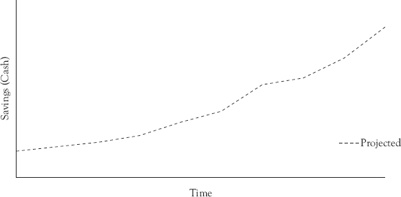
Figure 8.7 With all key information regarding the timing of management action and anticipated changes to cash_IN and cash_OUT, we can project rate of cash value realization

Key Takeaways

¹ H. Courtney. 2001. 20/20 Foresight: Crafting Strategy in an Uncertain World (1st ed.). Harvard Business School Press.