![]()
Solving Regression Problems in Machine Learning Using Sklearn Library
Machine learning is a branch of artificial intelligence that enables computer programs to automatically learn and improve from experience. Machine learning algorithms learn from datasets, and then based on the patterns identified from the datasets, make predictions on unseen data.
Machine learning algorithms can be mainly categorized into two types: supervised learning algorithms and unsupervised learning algorithms.
Supervised machine learning algorithms are those algorithms where the input dataset and the corresponding output or true prediction are available, and the algorithms try to find the relationship between the inputs and outputs.
In unsupervised machine learning algorithms, however, the true labels for the outputs are not known. Rather, the algorithms try to find similar patterns in the data. Clustering algorithms are a typical example of unsupervised learning.
Supervised learning algorithms are divided further into two types: regression algorithms and classification algorithms.
Regression algorithms predict a continuous value, for example, the price of a house, blood pressure of a person, and a student’s score in a particular exam. Classification algorithms, on the flip side, predict a discrete value such as whether or not a tumor is malignant, whether a student is going to pass or fail an exam, etc.
In this chapter, you will study how machine learning algorithms can be used to solve regression problems, i.e., predict a continuous value using the Sklearn library (https://bit.ly/2Zvy2Sm). In chapter 7, you will see how to solve classification problems via Sklearn. The 8th chapter gives an overview of the unsupervised learning algorithm.
6.1. Preparing Data for Regression Problems
Machine learning algorithms require data to be in a certain format before the algorithms can be trained on the data. In this section, you will see various data preprocessing steps that you need to perform before you can train machine learning algorithms using the Sklearn library.
You can read data from CSV files. However, the datasets we are going to use in this section are available by default in the Seaborn library. To view all the datasets, you can use the get_dataset_names() function as shown in the following script:
Script 1:
1. import pandas as pd
2. import numpy as np
3. import seaborn as sns
4. sns.get_dataset_names()
Output:
[‘anagrams’,
‘anscombe’,
‘attention’,
‘brain_networks’,
‘car_crashes’,
‘diamonds’,
‘dots’,
‘exercise’,
‘flights’,
‘fmri’,
‘gammas’,
‘geyser’,
‘iris’,
‘mpg’,
‘penguins’,
‘planets’,
‘tips’,
‘titanic’]
To read a particular dataset into the Pandas dataframe, pass the dataset name to the load_dataset() method of the Seaborn library.
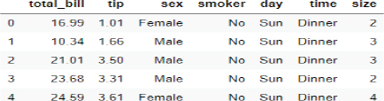
The following script loads the Tips dataset and displays its first five rows.
Script 2:
1. tips_df = sns.load_dataset(“tips”)
2. tips_df.head()
Output:
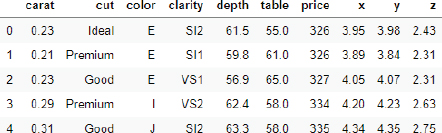
Similarly, the following script loads the Diamonds dataset and displays its first five rows.
Script 3:
1. diamond_df = sns.load_dataset(“diamonds”)
2. diamond_df.head()
Output:
In this chapter, we will be working with the Tips dataset. We will be using machine learning algorithms to predict the “tip” for a particular record, based on the remaining features such as “total_bill,” “sex,” “day,” “time,” etc.
6.1.1. Dividing Data into Features and Labels
As a first step, we divide the data into features and labels sets. Our labels set consists of values from the “tip” column, while the features set consists of values from the remaining columns. The following script divides the data into features and labels sets.
Script 4:
1. X = tips_df.drop([‘tip’], axis=1)
2. y = tips_df[“tip”]
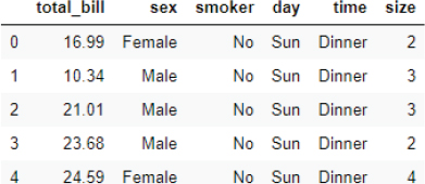
Let’s print the feature set.
Script 5:
1. X.head()
Output:
And the following script prints the label set.
Script 6:
1. y.head()
Output:
| 0 | 1.01 |
| 1 | 1.66 |
| 2 | 3.50 |
| 3 | 3.31 |
| 4 | 3.61 |
| Name: | tip, dtype: float64 |
6.1.2. Converting Categorical Data to Numbers
Machine learning algorithms, for the most part, can only work with numbers. Therefore, it is important to convert categorical data into a numeric format.
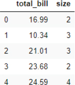
In this regard, the first step is to create a dataset of all numeric values. To do so, drop the categorical columns from the dataset, as shown below.
Script 7:
numerical = X.drop([‘sex’, ‘smoker’, ‘day’, ‘time’], axis = 1)
The output below shows that the dataframe “numerical” contains numeric columns only.
Script 8:
1. numerical.head()
Output:
Next, you need to create a dataframe that contains only categorical columns.
Script 9:
1. categorical = X.filter([‘sex’, ‘smoker’, ‘day’, ‘time’])
2. categorical.head()
Output:

One of the most common approaches to convert a categorical column to a numeric one is via one-hot encoding. In one-hot encoding, for every unique value in the original columns, a new column is created. For instance, for sex, two columns: Female and Male, are created. If the original sex column contained male, a 1 is added in the newly created Male column, while 1 is added in the newly created Female column if the original sex column contained Female.
However, it can be noted that we do not really need two columns. A single column, i.e., Female is enough since when a customer is female, we can add 1 in the Female column, else 1 can be added in that column. Hence, we need N-1 one-hot encoded columns for all the N values in the original column.
The following script converts categorical columns into one-hot encoded columns using the pd.get_dummies() method.
Script 10:
1. import pandas as pd
2. cat_numerical = pd.get_dummies(categorical,drop_first=True)
3. cat_numerical.head()
The output shows the newly created one-hot encoded columns.
Output:

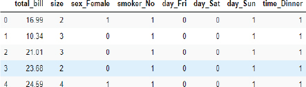
The final step is to join the numerical columns with the one-hot encoded columns. To do so, you can use the concat() function from the Pandas library as shown below:
Script 11:
1. X = pd.concat([numerical, cat_numerical], axis = 1)
2. X.head()
The final dataset looks like this. You can see that it doesn’t contain any categorical value.
Output:
6.1.3. Divide Data into Training and Test Sets
After you train a machine learning algorithm, you need to evaluate it to see how well it performs on unseen data. Therefore, we divide the dataset into two sets, i.e., a training set and a test set. The dataset is trained via the training set and evaluated on the test set. To split the data into training and test sets, you can use the train_test_split() function from the Sklearn library, as shown below. The following script divides the data into an 80 percent training set and a 20 percent test set.
Script 12:
1. from sklearn.model_selection import train_test_split
2.
3. X_train, X_test, y_train, y_test = train_test_split(X, y, test_size=0.20, random_state=0)
6.1.4. Data Scaling/Normalization
The final step (optional) before the data is passed to machine learning algorithms is to scale the data. You can see that some columns of the dataset contain small values, while the others contain very large values. It is better to convert all values to a uniform scale. To do so, you can use the StandardScaler() function from the sklearn.preprocessing module, as shown below:
Script 13:
1. from sklearn.preprocessing import StandardScaler
2. sc = StandardScaler()
3. #scaling the training set
4. X_train = sc.fit_transform(X_train)
5. #scaling the test set
6. X_test = sc.transform (X_test)
We have converted the data into a format that can be used to train machine learning algorithms for regression from the Sklearn library. The details, including functionalities and usage of all the machine learning algorithms, are available at this link. You can check all the regression algorithms by going to that link.
In the following section, we will review some of the most commonly used regression algorithms.
6.2. Linear Regression
Linear regression is a linear model that presumes a linear relationship between inputs and outputs and minimizes the cost of error between the predicted and actual output using functions like mean absolute error between different data points.
Why Use Linear Regression Algorithm?
The random forest algorithm is particularly useful when:
1.Linear regression is a simple to implement and easily interpretable algorithm.
2.Takes less training time to train even for huge datasets.
3.Linear regression coefficients are easy to interpret.
Disadvantages of Linear Regression Algorithm
The following are the disadvantages of the linear regression algorithm.
1.Performance is easily affected by outlier presence.
2.Assumes a linear relationship between dependent and independent variables, which can result in an increased error.
Implementing Linear Regression with Sklearn
To implement linear regression with Sklearn, you can use the LinearRegression class from the sklearn.linear_model module. To train the algorithm, the training and test sets, i.e., X_train and X_test in our case, are passed to the fit() method of the object of the LinearRegression class. The test set is passed to the predict() method of the class to make predictions. The process of training and making predictions with the linear regression algorithm is as follows:
Script 14:
1. from sklearn.linear_model import LinearRegression
2. # training the algorithm
3. lin_reg = LinearRegression()
4. regressor = lin_reg.fit(X_train, y_train)
5. # making predictions on test set
6. y_pred = regressor.predict(X_test)
Once you have trained a model and have made predictions on the test set, the next step is to know how well has your model performed for making predictions on the unknown test set. There are various metrics to check that. However, mean absolute error, mean squared error, and root mean squared error are three of the most common metrics.
Mean Absolute Error
Mean absolute error (MAE) is calculated by taking the average of absolute error obtained by subtracting real values from predicted values. The equation for calculating MAE is:

Mean Squared Error
Mean squared error (MSE) is similar to MAE. However, error for each record is squared in the case of MSE in order to punish data records with a huge difference between predicted and actual values. The equation to calculate the mean squared error is as follows:
![]()
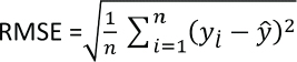
Root Mean Squared Error
Root Mean Squared Error is simply the under root of mean squared error and can be calculated as follows:
The methods used to find the value for these metrics are available in sklearn.metrics class. The predicted and actual values have to be passed to these methods, as shown in the output.
Script 15:
1. from sklearn import metrics
2.
3. print(‘Mean Absolute Error:’, metrics.mean_absolute_error(y_test, y_pred))
4. print(‘Mean Squared Error:’, metrics.mean_squared_error(y_test, y_pred))
5. print(‘Root Mean Squared Error:’, np.sqrt(metrics.mean_squared_error(y_test, y_pred)))
Here is the output. By looking at the mean absolute error, it can be concluded that on average, there is an error of 0.70 for predictions, which means that on average, the predicted tip values are 0.70$ more or less than the actual tip values.
Output:
Mean Absolute Error: 0.7080218832979829
Mean Squared Error: 0.893919522160961
Root Mean Squared Error: 0.9454731736865732
| Further Readings – Linear Regression |
| To study more about linear regression, please check these links: 1. https://bit.ly/2ZyCa49 2. https://bit.ly/2RmLhAp |
6.3. KNN Regression
KNN stands for K-nearest neighbors. KNN is a lazy learning algorithm, which is based on finding Euclidean distance between different data points.
Why Use KNN Algorithm?
The KNN is particularly useful when:
1.KNN Algorithm doesn’t assume any relationship between the features.
2.Useful for a dataset where data localization is important.
3.Only have to tune the parameter K, which is the number of nearest neighbors.
4.No training is needed, as it is a lazy learning algorithm.
5.Recommender systems and finding semantic similarity between the documents are major applications of the KNN algorithm.
Disadvantages of the KNN Algorithm
The following are the disadvantages of KNN algorithm.
1.You have to find the optimal value for K, which is not easy.
2.Not suitable for very high dimensional data.
Implementing the KNN Algorithm with SKlearn
With Sklearn, it is extremely easy to implement KNN regression. To do so, you can use the KNeighborsRegressor class. The process of training and testing is the same as linear regression. For training, you need to call the fit() method, and for testing, you need to call the predict() method.
The following script shows the process of training, testing, and evaluating the KNN regression algorithm for predicting the values for the tip column from the Tips dataset.
Script 16:
1. from sklearn.neighbors import KNeighborsRegressor
2. KNN_reg = KNeighborsRegressor(n_neighbors=5)
3. regressor = KNN_reg.fit(X_train, y_train)
4.
5. y_pred = regressor.predict(X_test)
6.
7.
8. from sklearn import metrics
9.
10. print(‘Mean Absolute Error:’, metrics.mean_absolute_error(y_test, y_pred))
11. print(‘Mean Squared Error:’, metrics.mean_squared_error(y_test, y_pred))
12. print(‘Root Mean Squared Error:’, np.sqrt(metrics.mean_squared_error(y_test, y_pred)))
Output:
Mean Absolute Error: 0.7513877551020406
Mean Squared Error: 0.9462902040816326
Root Mean Squared Error: 0.9727744877830794
| Further Readings – KNN Regression |
| To study more about KNN regression, please check these links: 1. https://bit.ly/35sIu0M 2. https://bit.ly/33r2Zbq |
6.4. Random Forest Regression
Random forest is a tree-based algorithm that converts features into tree nodes and then uses entropy loss to make predictions.
Why Use Random Forest Algorithms?
Random forest algorithms are particularly useful when:
1.You have lots of missing data or an imbalanced dataset.
2.With large number of trees, you can avoid overfitting while training. Overfitting occurs when machine learning models perform better on the training set but worse on the test set.
3.The random forest algorithm can be used when you have very high dimensional data.
4.Through cross-validation, the random forest algorithm can return higher accuracy.
5.The random forest algorithm can solve both classification and regression tasks and finds its application in a variety of tasks ranging from credit card fraud detection, stock market prediction, and finding fraudulent online transactions.
Disadvantages of Random Forest Algorithms
There are two major disadvantages of Random forest algorithms:
1.Using a large number of trees can slow down the algorithm.
2.Random forest algorithm is a predictive algorithm, which can only predict the future and cannot explain what happened in the past using the dataset.
Implementing Random Forest Regressor Using Sklearn
RandomForestRegressor class from the Sklearn.ensemble module can be used to implement random forest regressor algorithms, as shown below.
script 17:
1. # training and testing the random forest
2. from sklearn.ensemble import RandomForestRegressor
3. rf_reg = RandomForestRegressor(random_state=42, n_estimators=500)
4. regressor = rf_reg.fit(X_train, y_train)
5. y_pred = regressor.predict(X_test)
6.
7. # evaluating algorithm performance
8. from sklearn import metrics
9.
10. print(‘Mean Absolute Error:’, metrics.mean_absolute_error(y_test, y_pred))
11. print(‘Mean Squared Error:’, metrics.mean_squared_error(y_test, y_pred))
12. print(‘Root Mean Squared Error:’, np.sqrt(metrics.mean_squared_error(y_test, y_pred)))
The mean absolute error value of 0.70 shows that random forest performs better than both linear regression and KNN for predicting tip in the Tips dataset.
Output:
Mean Absolute Error: 0.7054065306122449
Mean Squared Error: 0.8045782841306138
Root Mean Squared Error: 0.8969828783932354
| Further Readings – Random Forest Regression |
| To study more about Random Forest Regression, please check these links: 1. https://bit.ly/3bRkKEy 2. https://bit.ly/35u3BzH |
6.5. Support Vector Regression
The support vector machine is classification as well as regression algorithms, which minimizes the error between the actual predictions and predicted predictions by maximizing the distance between hyperplanes that contain data for various records.
Why Use SVR Algorithms?
Support Vector Regression is a support vector machine (SVM) variant for regression. SVM has the following usages.
1.It can be used to perform regression or classification with high dimensional data.
2.With the kernel trick, SVM is capable of applying regression and classification to non-linear datasets.
3.SVM algorithms are commonly used for ordinal classification or regression, and this is why they are commonly known as ranking algorithms.
Disadvantages of SVR Algorithms
There are three major disadvantages of SVR algorithms:
1.Lots of parameters to be optimized in order to get the best performance.
2.Training can take a long time on large datasets.
3.Yields poor results if the number of features is greater than the number of records in a dataset.
Implementing SVR Using Sklearn
With the Sklearn library, you can use the SVM class to implement support vector regression algorithms, as shown below.
Script 18:
1. # training and testing the SVM
2.
3. from sklearn import svm
4. svm_reg = svm.SVR()
5.
6. regressor = svm_reg.fit(X_train, y_train)
7. y_pred = regressor.predict(X_test)
8.
9.
10. from sklearn import metrics
11.
12. print(‘Mean Absolute Error:’, metrics.mean_absolute_error(y_test, y_pred))
13. print(‘Mean Squared Error:’, metrics.mean_squared_error(y_test, y_pred))
14. print(‘Root Mean Squared Error:’, np.sqrt(metrics.mean_squared_error(y_test, y_pred)))
Mean Absolute Error: 0.7362521512772694
Mean Squared Error: 0.9684825097223093
Root Mean Squared Error: 0.9841150896731079
| Further Readings – Support Vector Regression |
| To study more about support vector regression, please check these links: 1. https://bit.ly/3bRACH9 2. https://bit.ly/3mg5PZG |
Which Model to Use?
The results obtained from section 6.2 to 6.5 shows that Random Forest Regressor algorithms result in the minimum MAE, MSE, and RMSE values. The algorithm you choose to use depends totally upon your dataset and evaluation metrics. Some algorithms perform better on one dataset while other algorithms perform better on the other dataset. It is better that you use all the algorithms to see, which gives the best results. However, if you have limited options, it is best to start with ensemble learning algorithms such as Random Forest. They yield the best result.
6.6. K Fold Cross-Validation
Earlier, we divided the data into an 80 Percent training set and a 20 percent test set. However, it means that only 20 percent of the data is used for testing and that 20 percent of data is never used for training.
For more stable results, it is recommended that all the parts of the dataset are used at least once for training and once for testing. The K-Fold cross-validation technique can be used to do so. With K-fold cross-validation, the data is divided into K parts. The experiments are also performed for K parts. In each experiment, K-1 parts are used for training, and the Kth part is used for testing.
For example, in 5-fold cross-validation, the data is divided into five equal parts, e.g., K1, K2, K3, K4, and K5. In the first iteration, K1–K4 are used for training, while K5 is used for testing. In the second test, K1, K2, K3, and K5 are used for training, and K4 is used for testing. In this way, each part is used at least once for testing and once for training.
You can use cross_val_score() function from the sklearn. model_selection module to perform cross validation as shown below:
Script 19:
1. from sklearn.model_selection import cross_val_score
2.
3. print(cross_val_score(regressor, X, y, cv=5, scoring =”neg_mean_absolute_error”))
Output:
[-0.66386205 -0.57007269 -0.63598762 -0.96960743 -0.87391702]
The output shows the mean absolute value for each of the K folds.
6.7. Making Prediction on a Single Record
In the previous sections, you saw how to make predictions on a complete test set. In this section, you will see how to make a prediction using a single record as an input.
Let’s pick the 100th record from our dataset.
Script 20:
1. tips_df.loc[100]
The output shows that the value of the tip in the 100th record in our dataset is 2.5.
Output:
| total_bill | 11.35 |
| tip | 2.5 |
| sex | Female |
| smoker | Yes |
| day | Fri |
| time | Dinner |
| size | 2 |
| Name: | 100, dtype: object |
We will try to predict the value of the tip of the 100th record using the random forest regressor algorithm and see what output we get. Look at the script below:
Note that you have to scale your single record before it can be used as input to your machine learning algorithm.
Script 21:
1. from sklearn.ensemble import RandomForestRegressor
2. rf_reg = RandomForestRegressor(random_state=42, n_estimators=500)
3. regressor = rf_reg.fit(X_train, y_train)
4.
5. single_record = sc.transform (X.values[100].reshape(1, -1))
6. predicted_tip = regressor.predict(single_record)
7. print(predicted_tip)
Output:
[2.2609]
The predicted value of the tip is 2.26, which is pretty close to 2.5, i.e., the actual value.
In the next chapter, you will see how to solve classification problems using machine learning algorithms in Scikit (Sklearn) library.
| Hands-on Time – Exercise |
| Now, it is your turn. Follow the instructions in the exercises below to check your understanding of the regression algorithms in machine learning. The answers to these exercises are provided after chapter 10 in this book. |
Exercise 6.1
Question 1
Among the following, which one is an example of a regression output?
A.True
B.Red
C.2.5
D.None of the above
Question 2
Which of the following algorithm is a lazy algorithm?
A.Random Forest
B.KNN
C.SVM
D.Linear Regression
Question 3
Which of the following algorithm is not a regression metric?
A.Accuracy
B.Recall
C.F1 Measure
D.All of the above
Exercise 6.2
Using the Diamonds dataset from the Seaborn library, train a regression algorithm of your choice, which predicts the price of the diamond. Perform all the preprocessing steps.