![]()
Solving Classification Problems in Machine Learning Using Sklearn Library
In the previous chapter, you saw how to solve regression problems with machine learning using the Sklearn library (https://bit.ly/2Zvy2Sm). In this chapter, you will see how to solve classification problems. Classification problems are the type of problems where you have to predict a discrete value, i.e., whether or not a tumor is malignant, if the condition of a car is good, whether or not a student will pass an exam, and so on.
7.1. Preparing Data for Classification Problems
Like regression, you have to first convert data into a specific format before it can be used to train classification algorithms.
The following script imports the Pandas, Seaborn, and NumPy libraries.
Script 1:
1. import pandas as pd
2. import numpy as np
3. import seaborn as sns
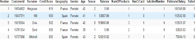
The following script uses the read_csv() method from the Pandas library to read the customer_churn.csv file, which contains records of customers who left the bank six months after various information about them is recorded. The head() method prints the first five rows of the dataset.
Script 2:
1. churn_df = pd.read_csv(“E:Hands on Python for Data Science and Machine LearningDatasetscustomer_churn.csv”)
2. churn_df.head()
The output shows that the dataset contains information such as surname, customer id, geography, gender, age, etc., as shown below. The Exited column contains information regarding whether or not the customer exited the bank after six months.
Output:
We do not need RowNumber, CustomerId, and Surname columns in our dataset since they do not help in predicting if a customer will churn or not. To remove these columns, you can use the drop() method, as shown below:
Script 3:
1. churn_df = churn_df.drop([‘RowNumber’, ‘CustomerId’, ‘Surname’], axis=1)
7.1.1. Dividing Data into Features and Labels
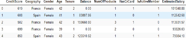
As shown in regression, the next step in classification is to divide the data into the features and labels. The features set, i.e., X in the following script contains all the columns except the Exited column. On the other hand, the labels set, i.e., y, contains values from the Exited column only.
Script 4:
1. X = churn_df.drop([‘Exited’], axis=1)
2. y = churn_df[‘Exited’]
The following script prints the first five rows of the feature set.
Script 5:
1. X.head()
Output:
And the following script prints the first five rows of the label set, as shown below:
Script 6:
1. y.head()
Output:
0 1
1 0
2 1
3 0
4 0
Name: Exited, dtype: int64
7.1.2. Converting Categorical Data to Numbers
In Section 6.1.2, you saw that we converted categorical columns to numerical because the machine learning algorithms in the Sklearn library only work with numbers.
For the classification problem, too, we need to convert the categorical column to numerical ones.
The first step then is to create a dataframe containing only numeric values. You can do so by dropping the categorical column and creating a new dataframe.
Script 7:
1. numerical = X.drop([‘Geography’, ‘Gender’], axis = 1)
The following script prints the dataframe that contains numeric columns only.
Script 8:
1. numerical.head()
Output:

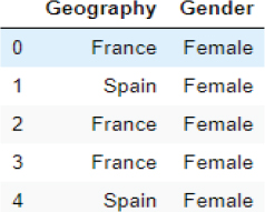
Next, create a dataframe that contains categorical values only. You can do so by using the filter() function as shown below:
Script 9:
1. categorical = X.filter([‘Geography’, ‘Gender’])
2. categorical.head()
The output shows that there are two categorical columns: Geography and Gender in our dataset.
Output:
In the previous chapter, you saw how to use the one-hot encoding approach in order to convert categorical features to numeric ones. Here, we will use the same approach:
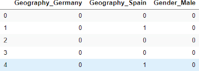
The following script converts categorical columns into one-hot encoded columns using the pd.get_dummies() method.
Script 10:
1. import pandas as pd
2. cat_numerical = pd.get_dummies(categorical,drop_first=True)
3. cat_numerical.head(
Output:
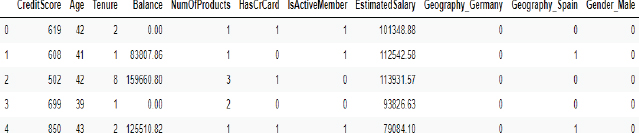
The last and final step is to join or concatenate the numeric columns and one-hot encoded categorical columns. To do so, you can use the concat function from the Pandas library, as shown below:
Script 11:
1. X = pd.concat([numerical, cat_numerical], axis = 1)
2. X.head()
The final dataset containing all the values in numeric form is shown here:
Output:
7.1.3. Divide Data into Training and Test Sets
After you train a machine learning algorithm, you need to evaluate it to see how well it performs on unseen data. Like regression, in classification problems, too, we divide the dataset into two sets, i.e., the training set and test set. The dataset is trained via the training set and evaluated on the test set. To split the data into training and test sets, you can use the train_test_split() function from the Sklearn library, as shown below. The following script divides the data into an 80 percent training set and a 20 percent test set.
Script 12:
1. from sklearn.model_selection import train_test_split
2. # test size is the fraction of test size
3. X_train, X_test, y_train, y_test = train_test_split(X, y, test_size=0.20, random_state=0)
7.1.4. Data Scaling/Normalization
The last step (optional) before data is passed to the machine learning algorithms is to scale the data. You can see that some columns of the dataset contain small values, while the other columns contain very large values. It is better to convert all values to a uniform scale. To do so, you can use the StandardScaler() function from the sklearn.preprocessing module, as shown below:
Script 13:
1. from sklearn.preprocessing import StandardScaler
2. sc = StandardScaler()
3. X_train = sc.fit_transform(X_train)
4. X_test = sc.transform (X_test)
We have converted data into a format that can be used to train machine learning algorithms for classification from the Sklearn library. The details, including functionalities and usage of all the machine learning algorithms, are available at this link. You can check all the classification algorithms by going to that link.
In the following section, we will review some of the most commonly used classification algorithms.
7.2. Logistic Regression
Logistic regression is a linear model which makes classification by passing the output of linear regression through a sigmoid function. The pros and cons of logistic regression algorithms are the same as linear regression algorithm explained already in chapter 6, section 6.2.
To implement linear regression with Sklearn, you can use the LogisticRegression class from the sklearn.linear_model module. To train the algorithm, the training and test sets, i.e., X_train and X_test in our case, are passed to the fit() method of the object of the LogisticRegression class. The test set is passed to the predict() method of the class to make predictions. The process of training and making predictions with the linear regression algorithm is as follows:
Script 14:
1. from sklearn.linear_model import LogisticRegression
2.
3. log_clf = LogisticRegression()
4. classifier = log_clf.fit(X_train, y_train)
5.
6. y_pred = classifier.predict(X_test)
7.
8.
Once you have trained a model and have made predictions on the test set, the next step is to know how well your model has performed for making predictions on the unknown test set. There are various metrics to evaluate a classification method. Some of the most commonly used classification metrics are F1, recall, precision, accuracy, and confusion matrix. Before you see the equations for these terms, you need to understand the concept of true positive, true negative, false positive, and false negative outputs:
True Negatives: (TN/tn): True negatives are those output labels that are actually false, and the model also predicted them as false.
True Positive: True positives are those labels that are actually true and also predicted as true by the model.
False Negative: False negative are labels that are actually true but predicted as false by the machine learning models.
False Positive: Labels that are actually false but predicted as true by the model are called false positive.
One way to analyze the results of a classification algorithm is by plotting a confusion matrix such as the one shown below:
Confusion Matrix

Precision
Another way to analyze a classification algorithm is by calculating precision, which is basically obtained by dividing true positives by the sum of true positive and false positive, as shown below:
![]()
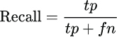
Recall
Recall is calculated by dividing true positives by the sum of the true positive and false negative, as shown below:
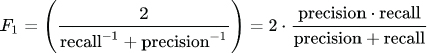
F1 Measure
F1 measure is simply the harmonic mean of precision and recall and is calculated as follows:
Accuracy
Accuracy refers to the number of correctly predicted labels divided by the total number of observations in a dataset.

The choice of using a metric for a classification problem depends totally upon you. However, as a rule of thumb, in case of balanced datasets, i.e., where the number of labels for each class is balanced, accuracy can be used as an evaluation metric. For imbalanced datasets, you can use F1 the measure as the classification metric.
The methods used to find the value for these metrics are available in the sklearn.metrics class. The predicted and actual values have to be passed to these methods, as shown in the output.
Script 15:
9. from sklearn.metrics import classification_report, confusion_matrix, accuracy_score
10.
11. print(confusion_matrix(y_test,y_pred))
12. print(classification_report(y_test,y_pred))
13. print(accuracy_score(y_test, y_pred))
Output:
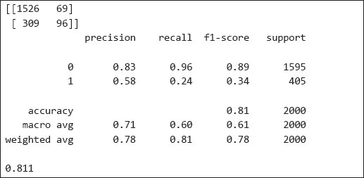
The output shows that for 81 percent of the records in the test set, logistic regression correctly predicted whether or not a customer will leave the bank.
| Further Readings – Logistic Regression |
| To study more about linear regression, please check these links: 1. https://bit.ly/3mjFV76 2. https://bit.ly/2FvcU7B |
7.3. KNN Classifier
As discussed in section 6.3, KNN stands for K-nearest neighbors. KNN is a lazy learning algorithm, which is based on finding Euclidean distance between different data points.
The pros and cons of the KNN classifier algorithm are the same as the KNN regression algorithm, which is explained already in Chapter 6, section 6.3.
KNN algorithm can be used both for classification and regression. With Sklearn, it is extremely easy to implement KNN classification. To do so, you can use the KNeighborsClassifiersclass.
The process of training and testing is the same as linear regression. For training, you need to call the fit() method, and for testing, you need to call the predict() method.
The following script shows the process of training, testing, and evaluating the KNN classification algorithm for predicting the values for the tip column from the Tips dataset.
Script 16:
1. from sklearn.neighbors import KNeighborsClassifier
2. knn_clf = KNeighborsClassifier(n_neighbors=5)
3. classifier = knn_clf.fit(X_train, y_train)
4.
5. y_pred = classifier.predict(X_test)
6.
7.
8. from sklearn.metrics import classification_report, confusion_matrix, accuracy_score
9.
10. print(confusion_matrix(y_test,y_pred))
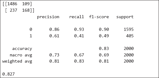
11. print(classification_report(y_test,y_pred))
12. print(accuracy_score(y_test, y_pred))
Output:
| Further Readings – KNN Classification |
| To study more about KNN classification, please check these links: 1. https://bit.ly/33pXWIj 2. https://bit.ly/2FqNmZx |
7.4. Random Forest Classifier
Like the random forest regressor, the random forest classifier is a tree-based algorithm that converts features into tree nodes, and then uses entropy loss to make classification predictions.
The pros and cons of the random forest classifier algorithm are the same as the random forest regression algorithm, which is explained already in Chapter 6, section 6.4.
RandomForestClassifier class from the Sklearn.ensemble module can be used to implement the random forest regressor algorithm in Python, as shown below.
Script 17:
1. from sklearn.ensemble import RandomForestClassifier
2. rf_clf = RandomForestClassifier(random_state=42, n_estimators=500)
3.
4. classifier = rf_clf.fit(X_train, y_train)
5.
6. y_pred = classifier.predict(X_test)
7.
8.
9. from sklearn.metrics import classification_report, confusion_matrix, accuracy_score
10.
11. print(confusion_matrix(y_test,y_pred))
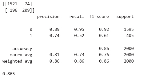
12. print(classification_report(y_test,y_pred))
13. print(accuracy_score(y_test, y_pred))
Output:
| Further Readings – Random Forest Classification |
| To study more about random forest classification, please check these links: 1. https://bit.ly/2V1G0k0 2. https://bit.ly/2GTyqDH |
7.5. Support Vector Classification
The support vector machine is classification as well as regression algorithms, which minimizes the error between the actual predictions and predicted predictions by maximizing the distance between hyperplanes that contain data for various records.
The pros and cons of the support vector classifier algorithm are the same as for the support vector regression algorithm, which is explained already in chapter 6, section 6.5.
With the Sklearn library, you can use the SVM module to implement the support vector classification algorithm, as shown below. The SVC class from the SVM module is used to implement the support vector classification, as shown below:
Script 18:
1. # training SVM algorithm
2. from sklearn import svm
3. svm_clf = svm.SVC()
4.
5. classifier = svm_clf .fit(X_train, y_train)
6. # making predictions on test set
7. y_pred = classifier.predict(X_test)
8.
# evaluating algorithm
9. from sklearn.metrics import classification_report, confusion_matrix, accuracy_score
10.
11. print(confusion_matrix(y_test,y_pred))
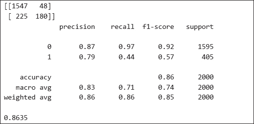
12. print(classification_report(y_test,y_pred))
13. print(accuracy_score(y_test, y_pred))
Output:
| Further Readings – SVM Classification |
| To study more about SVM classification, please check these links: 1. https://bit.ly/3hr4jAi 2. https://bit.ly/3iF0gln |
7.6. K-Fold Cross-Validation
You can also perform K-fold cross-validation for classification models, just like regression models. You can use cross_val_score() function from the sklearn.model_selection module to perform cross- validation, as shown below. For the classification algorithm, you need to pass a classification metric, e.g., accuracy to the scoring attribute.
Script 19:
1. from sklearn.model_selection import cross_val_score 2.
3. print(cross_val_score(classifier, X, y, cv=5, scoring =”accuracy”))
Output:
[0.796 0.796 0.7965 0.7965 0.7965]
7.7. Predicting a Single Value
Let’s make a prediction on a single customer record and see if he will leave the bank after six months or not.
The following script prints details of the 100th record.
Script 20:
1. churn_df.loc[100]
Output:
| CreditScore | 665 |
| Geography | France |
| Gender | Female |
| Age | 40 |
| Tenure | 6 |
| Balance | 0 |
| NumOfProducts | 1 |
| HasCrCard | 1 |
| IsActiveMember | 1 |
| EstimatedSalary | 161848 |
| Exited | 0 |
| Name: 100, dtype: | object |
The output above shows that the customer did not exit the bank after six months since the value for the Exited attribute is 0. Let’s see what our classification model predicts:
Script 21:
1. # training the random forest algorithm
2. from sklearn.ensemble import RandomForestClassifier
3. rf_clf = RandomForestClassifier(random_state=42, n_estimators=500)
4.
5. classifier = rf_clf.fit(X_train, y_train)
6.
7. # scaling single record
8. single_record = sc.transform (X.values[100].reshape(1, -1))
9.
10. #making predictions on the single record
11. predicted_churn = classifier.predict(single_record)
12. print(predicted_churn)
The output is 0, which shows that our model correctly predicted that the customer will not churn after six months.
Output:
[0]
| Hands-on Time – Exercise |
| Now, it is your turn. Follow the instructions in the exercises below to check your understanding of the about classification algorithms in machine learning. The answers to these exercises are provided after chapter 10 in this book. |
Exercise 7.1
Question 1
Among the following, which one is not an example of classification outputs?
A.True
B.Red
C.Male
D.None of the above
Question 2
Which of the following metrics is used for unbalanced classification datasets?
A.Accuracy
B.F1
C.Precision
D.Recall
Question 3
Among the following functions, which one is used to convert categorical values to one-hot encoded numerical values?
A.pd.get_onehot()
B.pd.get_dummies()
C.pd.get_numeric()
D.All of the above
Exercise 7.2
Using the iris dataset from the Seaborn library, train a classification algorithm of your choice, which predicts the species of the iris plant. Perform all the preprocessing steps.