Deep Learning with Python TensorFlow 2.0

In this chapter, you will be using TensorFlow 2.0 and Keras API to implement different types of neural networks in Python. From TensorFlow 2.0, Google has officially adopted Keras as the main API to run TensorFlow scripts.

In this chapter, you will study three different types of Neural Networks: Densely Connected Neural Network, Recurrent Neural Network, and Convolutional Neural Network, with TensorFlow 2.0.

9.1. Densely Connected Neural Network

A densely connected neural network (DNN) is a type of neural network where all the nodes in the previous layer are connected to all the nodes in the subsequent layer of a neural network. A DNN is also called a multilayer perceptron.

A densely connected neural network is mostly used for making predictions on tabular data. Tabular data is the type of data that can be presented in the form of a table.

In a neural network, we have an input layer, one or multiple hidden layers, and an output layer. An example of a neural network is shown below:

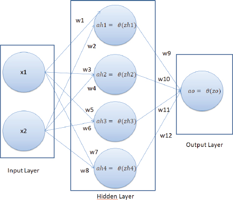
In our neural network, we have two nodes in the input layer (since there are two features in the input), one hidden layer with four nodes, and one output layer with one node since we are doing binary classification. The number of hidden layers, along with the number of neurons per hidden layer, depends upon you.

In the above neural network, the x1 and x2 are the input features, and the ao is the output of the network. Here, the only attribute we can control is the weights w1, w2, w3, ….. w12. The idea is to find the values of weights for which the difference between the predicted output ao in this case and the actual output (labels).

A neural network works in two steps:

1.Feed Forward

2.Backpropagation

I will explain both these steps in the context of our neural network.

9.1.1. Feed Forward

In the feed forward step, the final output of a neural network is created. Let’s try to find the final output of our neural network.

In our neural network, we will first find the value of zh1, which can be calculated as follows:

Using zh1, we can find the value of ah1, which is:

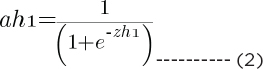
In the same way, you find the values of ah2, ah3, and ah4.

To find the value of zo, you can use the following formula:

Finally, to find the output of the neural network ao:

9.1.2. Backpropagation

The purpose of backpropagation is to minimize the overall loss by finding the optimum values of weights. The loss function we are going to use in this section is the mean squared error, which is in our case represented as:

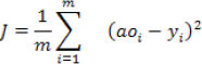
Here, ao is the predicted output from our neural network, and y is the actual output.

Our weights are divided into two parts. We have weights that connect input features to the hidden layer and the hidden layer to the output node. We call the weights that connect the input to the hidden layer collectively as wh (w1, w2, w3 …… w8), and the weights connecting the hidden layer to the output as wo (w9, w10, w11, w12).

The backpropagation will consist of two phases. In the first phase, we will find dcost/dwo (which refers to the derivative of the total cost with respect to wo, weights in the output layer). By the chain rule, dcost/dwo can be represented as the product of dcost/dao * dao/dzo * dzo/dwo. (d here refers to a derivative.) Mathematically:

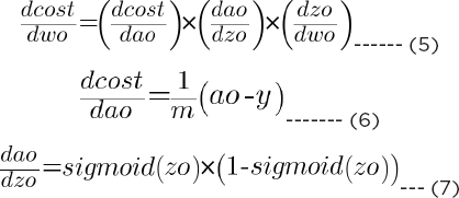
In the same way, you find the derivative of cost with respect to bias in the output layer, i.e., dcost/dbo, which is given as:

Putting 6, 7, and 8 in equation 5, we can get the derivative of cost with respect to the output weights.

The next step is to find the derivative of cost with respect to hidden layer weights wh and bias bh. Let’s first find the derivative of cost with respect to hidden layer weights:

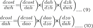
The values of dcost/dao and dao/dzo can be calculated from equations 6 and 7, respectively. The value of dzo/dah is given as:

Putting the values of equations 6, 7, and 11 in equation 11, you can get the value of equation 10.

Next, let’s find the value of dah/dzh:

and,

Using equation 10, 12, and 13 in equation 9, you can find the value of dcost/dwh.

9.1.3. Implementing a Densely Connected Neural Network

In this section, you will see how to implement a densely connected neural network with TensorFlow, which predicts whether or not a banknote is genuine or not, based on certain features such as variance, skewness, curtosis, and entropy of several banknote images. Let’s begin without much ado. The following script upgrades the existing TensorFlow version. I always recommend doing this.

Script 1:

To check if you are actually running TensorFlow 2.0, execute the following command.

Script 2:

You should see 2.x.x in the output, as shown below:

Output:

§ Importing Required Libraries

Let’s import the required libraries.

Script 3:

§ Importing the Dataset

The dataset that we are going to use can be downloaded free from the following GitHub resource. The dataset is also available by the name “banknotes.csv” in the Datasets folder in the GitHub repository.

Script 4:

The following script plots the first five rows of the dataset.

Script 5:

Output:

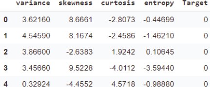
The output shows that our dataset contains five columns. Let’s see the shape of our dataset.

Script 6:

The output shows that our dataset has 1372 rows and 5 columns.

Output:

Let’s plot a count plot to see the distribution of data with respect to the values in the class that we want to predict.

Script 7:

Output:

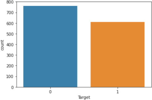
The output shows that the number of fake notes (represented by 1) is slightly less than the number of original banknotes.

The task is to predict the values for the “Target” column, based on the values in the first four columns. Let’s divide our data into features and target labels.

Script 8:

Output:

The variable X contains our feature set while the variable y contains target labels.

§ Dividing Data into Training and Test Sets

Deep learning models are normally trained on one set of data and are tested on another set. The dataset used to train a deep learning model is called a training set, and the dataset used to evaluate the performance of the trained deep learning model is called the test set.

We will divide the total data into an 80 percent training set and a 20 percent test set. The following script performs that task.

Script 9:

Before you train your deep learning model, it is always a good practice to scale your data. The following script applies standard scaling to the training and test sets.

Script 10:

§ Creating a Neural Network

To create a neural network, you can use the Sequential class from the tensorflow.keras.models module. To add layers to your model, you simply need to call the add method and pass your layer to it. To create a dense layer, you can use the Dense class.

The first parameter to the Dense class is the number of nodes in the dense layer, and the second parameter is the dimension of the input. The activation function can be defined by passing a string value to the activation attribute of the Dense class. It is important to mention that the input dimensions are only required to be passed to the first dense layer. The subsequent dense layers can calculate the input dimensions automatically from the number of nodes in the previous layers.

The following script defines a method create_model. The model takes two parameters: learning_rate and dropout_rate. Inside the model, we create an object of the Sequential class and add three dense layers to the model. The layers contain 12, 6, and 1 nodes, respectively. After each dense layer, we add a dropout layer with a dropout rate of 0.1. Adding dropout after each layer avoids overfitting. After you create the model,

you need to compile it via the compile method. The compile method takes the loss function, the optimizer, and the metrics as parameters. Remember, for binary classification, the activation function in the final dense layer will be sigmoid, whereas the loss function in the compile method will be binary_crossentropy.

Script 11:

Next, we need to define the default dropout rate, learning rate batch size, and the number of epochs. The number of epochs refers to the number of times the whole dataset is used for training, and the batch size refers to the number of records, after which the weights are updated.

The following script creates our model.

Script 12:

You can see your model architecture via the plot_model() method of the tensorflow.keras.utils module.

Script 13:

Output:

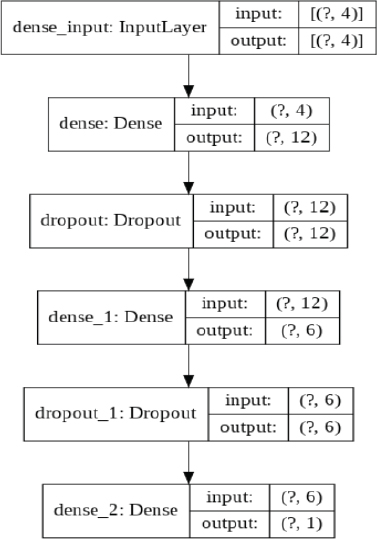
From the above output, you can see that the input layer contains four nodes, the input to the first dense layers is 4, while the output is 12. Similarly, the input to the second dense layer is 12, while the output is 6. Finally, in the last dense layer, the input is 6 nodes, while the output is 1 since we are making a binary classification. Also, you can see a dropout layer after each dense layer.

To train the model, you need to call the fit method on the model object. The fit method takes the training features and targets as parameters, along with the batch size, the number of epochs, and the validation split. The validation split refers to the split in the training data during training.

Script 14:

The result from the last five epochs is shown below:

Output:

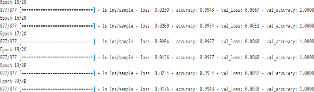
Our neural network is now trained. The “val_accuracy” of 1.0 in the last epoch shows that on the training set, our neural network is making predictions with 100 percent accuracy.

§ Evaluating the Neural Network Performance

We can now evaluate its performance by making predictions on the test set. To make predictions on the test set, you have to pass the set to the evaluate() method of the model, as shown below:

Script 15:

Output:

The output shows an accuracy of 100 percent on the test set. The loss value of 0.00397 is shown. Remember, lower the loss, higher the accuracy.

Let’s now plot the accuracy on the training and test sets to see if our model is overfitting or not.

Script 16:

Output:

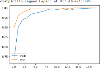
The above curve meets near 1 and then becomes stable which shows that our model is not overfitting.

Similarly, the loss values for test and training sets can be printed as follows:

Script 17:

Output:

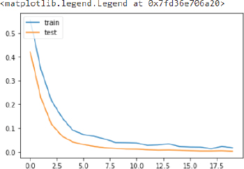
And this is it. You have successfully trained a neural network for classification. In the next section, you will see how to create and train a recurrent neural network for stock price prediction.

9.2. Recurrent Neural Networks (RNN)

9.2.1. What Is an RNN and LSTM?

This section explains what a recurrent neural network (RNN) is, what is the problem with RNN, and how a long short-term memory network (LSTM) can be used to solve the problems with RNN.

§ What Is an RNN?

A recurrent neural network is a type of neural network that is used to process data that is sequential in nature, e.g., stock price data, text sentences, or sales of items.

Sequential data is a type of data where the value of data at time step T depends upon the values of data at timesteps less than T. For instance, sound waves, text sentences, stock market prices, etc. In the stock market price prediction problem, the value of the opening price of a stock at a given data depends upon the opening stock price of the previous days.

The difference between the architecture of a recurrent neural network and a simple neural network is presented in the following figure:

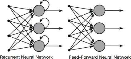
In a recurrent neural network, at each time step, the previous output of the neuron is also multiplied by the current input via a weight vector. You can see from the above figure that the output from a neuron is looped back into for the next time step. The following figure makes this concept further clear:

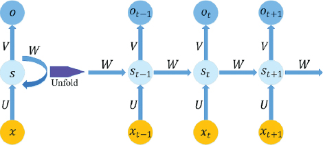
Here, we have a single neuron with one input and one output. On the right side, the process followed by a recurrent neural network is unfolded. You can see that at time step t, the input is multiplied by weight vector U, while the previous output at time t–1, i.e., St–1 is multiplied by the weight vector W, the sum of the input vector XU + SW becomes the output at time T. This is how a recurrent neural network captures the sequential information.

§ Problems with RNN

A problem with the recurrent neural network is that while it can capture a shorter sequence, it tends to forget longer sequences.

For instance, it is easier to predict the missing word in the following sentence because the Keyword “Birds” is present in the same sentence.

“Birds fly in the ___.”

RNN can easily guess that the missing word is “Clouds” here.

However, RNN cannot remember longer sequences such as the one …

“Mike grew up in France. He likes to eat cheese, he plays piano……………………………………………………………………………………….. and he speaks _______ fluently”.

Here, the RNN can only guess that the missing word is “French” if it remembers the first sentence, i.e., “Mike grew up in France.”

The recurrent neural networks consist of multiple recurrent layers, which results in a diminishing gradient problem. The diminishing gradient problem is that during the backpropagation of the recurrent layer, the gradient of the earlier layer becomes infinitesimally small, which virtually makes neural network initial layers stop from learning anything.

To solve this problem, a special type of recurrent neural network, i.e., Long Short-Term Memory (LSTM) has been developed.

§ What Is an LSTM?

LSTM is a type of RNN which is capable of remembering longer sequences, and hence, it is one of the most commonly used RNN for sequence tasks.

In LSTM, instead of a single unit in the recurrent cell, there are four interacting units, i.e., a forget gate, an input gate, an update gate, and an output gate. The overall architecture of an LSTM cell is shown in the following figure:

Let’s briefly discuss all the components of LSTM:

§ Cell State

The cell state in LSTM is responsible for remembering a long sequence. The following figure describes the cell state:

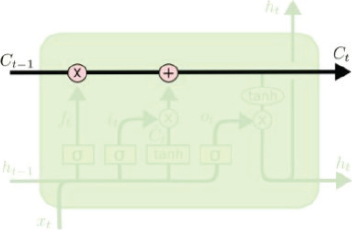
The cell state contains data from all the previous cells in the sequence. The LSTM is capable of adding or removing information to a cell state. In other words, LSTM tells the cell state which part of previous information to remember and which information to forget.

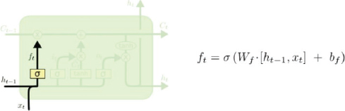
§ Forget Gate

The forget gate basically tells the cell state which information to retain from the information in the previous step and which information to forget. The working and calculation formula for the forget gate is as follows:

§ Input Gate

The forget gate is used to decide which information to remember or forget. The input gate is responsible for updating or adding any new information in the cell state. The input gate has two parts: an input layer, which decides which part of the cell state is to be updated, and a tanh layer, which actually creates a vector of new values that are added or replaced in the cell state. The working of the input gate is explained in the following figure:

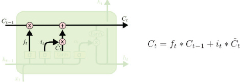
§ Update Gate

The forget gate tells us what to forget, and the input gate tells us what to add to the cell state. The next step is to actually perform these two operations. The update gate is basically used to perform these two operations. The functioning and the equations for the update gate are as follows:

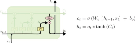
§ Output Gate

Finally, you have the output gate, which outputs the hidden state and the output, just like a common recurrent neural network. The additional output from an LSTM node is a cell state, which runs between all the nodes in a sequence. The equations and the functioning of the output gate are depicted by the following figure:

In the following sections, you will see how to use LSTM for solving different types of Sequence problems.

9.3. Predicting Future Stock Prices via LSTM in Keras

Stock price prediction is one of the most common applications of many to one or many to many sequence problems.

In this section, we will predict the opening stock price of the Facebook company, using the opening stock price of the previous 60 days. The training set consists of the stock price data of Facebook from 1^st January 2015 to 31^st December 2019, i.e., five years. The dataset can be downloaded from this site:

https://finance.yahoo.com/quote/FB/history?p=FB.

The test data will consist of the opening stock prices of the Facebook company for the month of January 2020. The training file fb_train.csv and the test file fb_test.csv are also available in the Datasets folder in the GitHub repository. Let’s begin with the coding now.

9.3.1. Training the Stock Prediction Model

In this section, we will train our stock prediction model on the training set.

Before you train the stock market prediction model, upload the TensorFlow version by executing the following command on Google collaborator (https://colab.research.google.com/).

Script 18:

If your files are placed on Google Drive, and you want to access them in Google Collaborator, to do so, you have to first mount the Google Drive inside your Google Collaborator environment via the following script:

Script 19:

Next, to import the training dataset, execute the following script:

Script 20:

Running the following script will print the first five rows of the dataset.

Script 21:

Output:

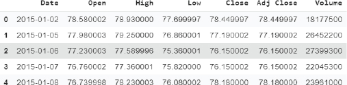
The output shows that our dataset consists of seven columns. However, in this section, we are only interested in the Open column. Therefore, we will select the Open column from the dataset. Run the following script to do so.

Script 22:

Next, we will scale our dataset.

Script 23:

If you check the total length of the dataset, you will see it has 1257 records, as shown below:

Script 24:

Output:

Before we proceed further, we need to divide our data into features and labels. Our feature set will consist of 60 timesteps of 1 feature. The feature set basically consists of the opening stock price of the past 60 days, while the label set will consist of the opening stock price of 61^st day. Based on the opening stock prices of the previous days, we will be predicted the opening stock price for the next day.

Script 25:

We need to convert our data into Numpy array before we can use as input with Keras. The following script does that:

Script 26:

Let’s print the shape of our dataset.

Script 27:

Output:

We need to reshape our input features into 3-dimensional format.

Script 28:

The following script creates our LSTM model. We have 4 LSTM layers with 100 nodes each. Each LSTM layer is followed by a dropout layer to avoid overfitting. The final dense has one node since the output is a single value.

Script 29:

Script 30:

Next, we need to convert the output y into a column vector.

Script 31:

Output:

The following script trains our stock price prediction model on the training set.

Script 32:

You can see the results for the last five epochs in the output.

Output:

Our model has been trained. Next, we will test our stock prediction model on the test data.

9.3.2. Testing the Stock Prediction Model

The test data should also be converted into the right shape to test our stock prediction model. We will do that later. Let’s first import the data and then remove all the columns from the test data except the Open column.

Script 33:

Let’s concatenate the training and test sets. We do this to predict the first value in the test set. The input will be the data from the past 60 days, which is basically the data from the last 60 days in the training set.

Script 34:

The following script creates our final input feature set.

Script 35:

You can see that the length of the input data is 80. Here, the first 60 records are the last 60 records from the training data, and the last 20 records are the 20 records from the test file.

Output:

We need to scale our data and convert it into a column vector.

Script 36:

Output:

As we did with the training data, we need to divide our input data into features and labels. Here is the script that does that.

Script 37:

Let’s now print our feature set.

Script 38:

Output:

Our feature set is currently 2-dimensional. But the LSTM algorithm in Keras accepts only data in 3-dimensional. The following script converts our input features into a 3-dimensional shape.

Script 39:

Output:

Now is the time to make predictions on the test set. The following script does that:

Script 40:

Since we scaled our input feature, we need to apply the inverse_transform() method of the scaler object on the predicted output to get the original output values.

Script 41:

Finally, to compare the predicted output with the actual stock price values, you can plot the two values via the following script:

Script 42:

Output:

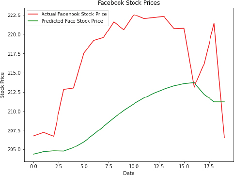
The output shows that our algorithm has been able to partially capture the trend of the future opening stock prices for Facebook data.

In the next section, you will see how to perform image classification using a convolutional neural network.

9.4. Convolutional Neural Network

A convolutional neural network is a type of neural network that is used to classify spatial data, for instance, images, sequences, etc. In an image, each pixel is somehow related to some other pictures. Looking at a single pixel, you cannot guess the image. Rather you have to look at the complete picture to guess the image. A CNN does exactly that. Using a kernel or feature detects, it detects features within an image. A combination of these images then forms the complete image, which can then be classified using a densely connected neural network. The steps involved in a Convolutional Neural Network have been explained in the next section.

9.4.1. Image Classification with CNN

In this section, you will see how to perform image classification using CNN. Before we go ahead and see the steps involved in the image classification using a convolutional neural network, we first need to know how computers see images.

§ How Do Computers See Images?

When humans see an image, they see lines, circles, squares, and different shapes. However, a computer sees an image differently. For a computer, an image is no more than a 2-D set of pixels arranged in a certain manner. For greyscale images, the pixel value can be between 0–255, while for color images, there are three channels: red, green, and blue. Each channel can have a pixel value between 0–255.

Look at the following image 9.1.

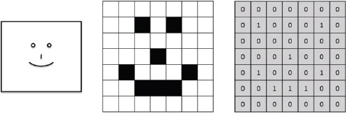
Image 9.1: How computers see images

Here, the box on the leftmost is what humans see. They see a smiling face. However, a computer sees it in the form of pixel values of 0s and 1s, as shown on the right-hand side. Here, 0 indicates a white pixel, whereas 1 indicates a black pixel. In the real-world, 1 indicates a white pixel, while 0 indicates a black pixel.

Now, we know how a computer sees images. The next step is to explain the steps involved in the image classification using a convolutional neural network.

The following are the steps involved in image classification with CNN:

1.The Convolution Operation

2.The ReLu Operation

3.The Pooling Operation

4.Filattening and Fully Connected Layer.

§ The Convolution Operation

The convolution operation is the first step involved in the image classification with a convolutional neural network.

In a convolution operation, you have an image and a feature detector. The values of the feature detector are initialized randomly. The feature detector is moved over the image from left to right. The values in the feature detector are multiplied by the corresponding values in the image, and then all the values in the feature detector are added. The resultant value is added to the feature map.

Look at the following image, for example:

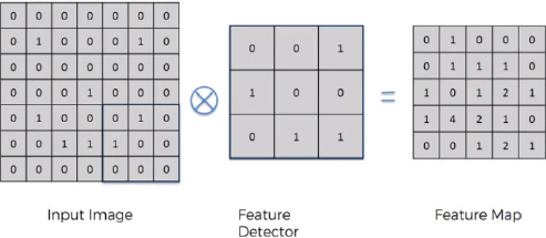
In the above image, we have an input image of 7 x 7. The feature detector is of the size 3 x 3. The feature detector is placed over the image at the top left of the input image, and then the pixel values in the feature detector are multiplied by the pixel values in the input image. The result is then added. The feature detector then moves to N step towards the right. Here, N refers to stride. A stride is basically the number of steps that a feature detector takes from left to right and then from top to bottom to find a new value for the feature map.

In reality, there are multiple feature detectors. As shown in the following image:

Each feature detector is responsible for detecting a particular feature in the image.

§ The ReLu Operation

In a ReLu operation, you simply apply the ReLu activation function on the feature map generated as a result of the convolution operation. A convolution operation gives us linear values. The ReLu operation is performed to introduce non-linearity in the image.

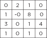
In the ReLu operation, all the negative values in a feature map are replaced by 0. All the positive values are left untouched.

Suppose we have the following feature map:

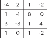
When the ReLu function is applied on the feature map, the resultant feature map looks like this:

§ The Pooling Operation

A pooling operation is performed in order to introduce spatial invariance in the feature map. Pooling operation is performed after convolution and ReLu operation.

Let’s first understand what spatial invariance is. If you look at the following three images, you can easily identify that these images contain cheetahs.

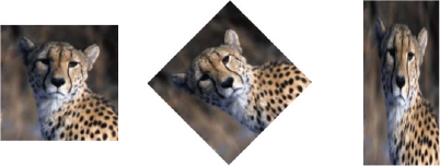
Here, the second image is disoriented, and the third image is distorted. However, we are still able to identify that all the three images contain cheetahs based on certain features.

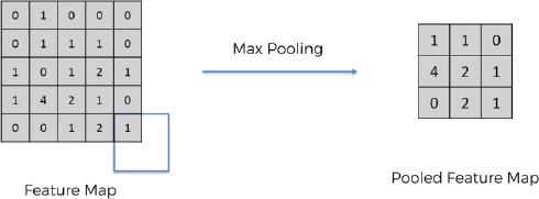
Pooling does exactly that. In pooling, we have a feature map and then a pooling filter, which can be of any size. Next, we move the pooling filter over the feature map and apply the pooling operation. There can be many pooling operations such as max pooling, min pooling, and average pooling. In max pooling, we choose the maximum value from the pooling filter. Pooling not only introduces spatial invariance but also reduces the size of an image.

Look at the following image. Here, in the 3^rd and 4^th rows and 1^st and 2nd columns, we have four values 1, 0, 1, and 4. When we apply max pooling on these four pixels, the maximum value will be chosen, i.e., you can see 4 in the pooled feature map.

§ Flattening and Fully Connected Layer

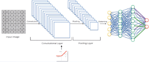
The pooled feature maps are flattened to form a one-dimensional vector to find more features from an image, as shown in the following figure:

The one-dimensional vector is then used as input to a densely or fully connected neural network layer that you saw in Chapter 4. This is shown in the following image:

9.4.2. Implementing CNN with TensorFlow Keras

In this section, you will see how to implement CNN for image classification in TensorFlow Keras. We will create CNN that is able to classify an image of fashion items such as shirt, pants, trousers, sandals into one of the 10 predefined categories. So, let’s begin without much ado.

Execute the following script to make sure that you are running the latest version of TensorFlow.

Script 43:

Output:

The following script imports the required libraries and classes.

Script 44:

The following script downloads the Fashion MNIST dataset that contains images of different fashion items along with their labels. The script divides the data into training images and training labels and test images and test labels.

Script 45:

The images in our dataset are greyscale images, where each pixel value lies between 0 and 255. The following script normalizes pixel values between 0 and 1.

Script 46:

Let’s print the shape of our training data.

Script 47:

Output:

The above output shows that our training dataset contains 60,000 records (images). Each image is 28 pixels wide and 28 pixels high.

Let’s print an image randomly from the test set:

Script 48:

Output:

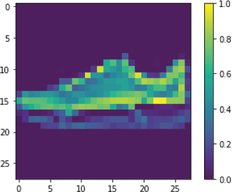
The output shows that the 9^th image in our test set is the image of a sneaker.

The next step is to change the dimensions of our input images. CNN in Keras expects data to be in the format Width-Height-Channels. Our images contain width and height but no channels. Since the images are greyscale, we set the image channel to 1, as shown in the following script:

Script 49:

Output:

The next step is to find the number of output classes. This number will be used to define the number of neurons in the output layer.

Script 50:

Output:

As expected, the number of the output classes in our dataset is 10.

Let’s print the shape of a single image in the training set.

Script 51:

Output:

The shape of a single image is (28, 28, 1). This shape will be used to train our convolutional neural network. The following script creates a model for our convolutional neural network.

Script 52:

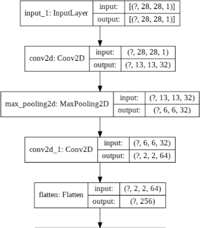
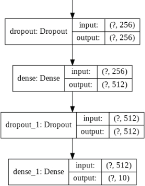
The model contains one input layer, two convolutional layers, one flattening layer, one hidden dense layer, in one output layer. The number of filters in the first convolutional layer is 32, while in the second convolutional layer, it is 64. The kernel size for both convolutional layers is 3 x 3, with a stride of 2. After the first convolutional layer, a max-pooling layer with a size 2 x 2 and stride 2 has also been defined.

It is important to mention that while defining the model layers, we used Keras Functional API. With Keras functional API, to connect the previous layer with the next layer, the name of the previous layer is passed inside the parenthesis at the end of the next layer.

The following line compiles the model.

Script 53:

Finally, execute the following script to print the model architecture.

Script 54:

Output:

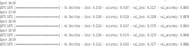
The following script trains the image classification model.

Script 55:

The results from the last five epochs are shown in the output.

Output:

Let’s plot the training and test accuracies for our model.

Script 56:

The following output shows that training accuracy is higher, and test accuracy starts to flatten after 88 percent. We can say that our model is overfitting.

Output:

Let’s make a prediction on one of the images in the test set. Let’s predict the label for image 9. We know that image 9 contains a sneaker, as we saw earlier by plotting the image.

Script 57:

Output:

The output shows number 7. The output will always be a number since deep learning algorithms work only with numbers. The numbers correspond to the following labels:

0: T-shirt op

1: Trousers

2: Pullover

3: Dress

4: Coat

5: Sandals

6: Shirt

7: Sneakers

8: Bag

9: Ankle boot

The above list shows that the number 7 corresponds to sneakers. Hence, the prediction by our CNN is correct.

In this chapter, you saw how to implement different types of deep neural networks, i.e., a densely connected neural network, a recurrent neural network, and a convolutional neural network with TensorFlow 2.0 and Keras library in Python.

Hands-on Time – Exercise

Now, it is your turn. Follow the instructions in the exercises below to check your understanding of the deep learning algorithms in TensorFlow 2.0. The answers to these exercises are provided after chapter 10 in this book.

Exercise 9.1

Question 1

What should be the input shape of the input image to the convolutional neural network?

A.Width, Height

B.Height, Width

C.Channels, Width, Height

D.Width, Height, Channels

Question 2

We say that a model is overfitting when:

A.Results on test set are better than train set

B.Results on both test and training sets are similar

C.Results on the training set are better than the results on the test set

D.None of the above

Question 3

The ReLu activation function is used to introduce:

A.Linearity

B.Non-linearity

C.Quadraticity

D.None of the above

Exercise 9.2

Using the CFAR 10 image dataset, perform image classification to recognize the image. Here is the dataset: