
5
Parameter Mixing in Infinite-server Queues
Lucas VAN KREVELD1 and Onno BOXMA2
1Korteweg-de Vries Institute, University of Amsterdam, The Netherlands
2Eindhoven University of Technology, The Netherlands
We consider two infinite-server queueing models with a so-called mixed arrival process. The arrival process is Poisson, but the arrival intensity is resampled from some distribution at exponentially distributed time intervals. First, we study the case of Coxian service times. For this infinite-server model, we show how to compute all joint moments of the arrival rate and the number of customers, both in transient and steady state. Second, we consider a Markov-modulated infinite-server queue with general service times. The arrival intensity is resampled at the state change epochs of the Markov background process. We develop a procedure to obtain all transient moments of the number of customers given the initial state and the initial arrival rate.
5.1. Introduction
In queueing theory, it is often assumed that the arrival process is a Poisson process with a constant rate. This is not always a realistic assumption, and hence various adaptations have been suggested to better reflect reality. We mention four types of adaptation, in which the arrival process still maintains essential elements and properties of the Poisson process. First, there have been studies of queues with time-inhomogeneous Poisson arrivals (Eick et al. 1993), and of queues with Markov-modulated arrivals in which the arrival process is Poisson with rate λi when some underlying Markov process is in state i (see Asmussen (2003, Ch. XI), and the pioneering work of Neuts (1981, 1989)). Second, there is a growing interest in queues with Cox arrival processes. These are Poisson processes in which the time-dependent arrival intensity, say Λ(t), itself is a stochastic process. The variance of the number of arrivals of a Cox process in a given interval is larger than the mean (whereas they are equal for Poisson); this phenomenon is usually called overdispersion. In a few papers, the process {Λ(t), t ≥ 0} was taken to be a shot-noise process. We refer to (Albrecher and Asmussen 2006) for an example in insurance mathematics and to (Koops et al. 2017) for a queueing example. Third, the so-called mixture models have been suggested. In such models, the arrival rate is itself a random variable with some distribution. In the queueing literature, it is not so common to consider mixing distributions (Jongbloed and Koole 2001), but this is different in the finance and insurance literature (e.g. Bühlmann (1972) already considered them in 1972 in the context of credibility-based dynamic premium rules). Recent studies of single-server queues with mixing include that of Raaijmakers et al. (2019) (in which the random parameter is sampled once and for all) and Klaasse (2017) (in which the random parameter is resampled in each new busy period). Fourth, we would like to mention the theory of switching processes, as developed by Anisimov. Such processes describe the operation of stochastic systems with the property that their development in time switches at some random points in time, which may depend on the past system trajectory. In (Anisimov 2008), Anisimov studies asymptotic results for large classes of switching processes.
One class of queueing models for which generalizations of the classical Poisson arrival process have been studied is the class of infinite-server models. Websites provide interesting applications of such systems (but there are many other applications). The arrival rate of website visits typically is not constant in time and could depend on an environment (Markov modulation), or vary according to some stochastic process that takes external events into account (e.g. shot-noise driven), or take a new random value after some time (mixing). Numerous variants of stochastic background processes in infinite-server queues have been studied after the pioneering paper of O’Cinneide and Purdue (1986). Jansen et al. (2016) have considered a general càdlàg stochastic process as background process, whereas D’Auria (2008), Anderson et al. (2016) and Blom et al. (2014) were restricted to the case where the background process is Markov. Next to the already mentioned case of an infinite-server model with a Coxian, shot-noise driven, arrival process (Koops et al. 2017), infinite-server systems with the more general Hawkes, or self-exciting, input process have recently been analyzed (Daw and Pender 2018; Koops et al. 2018).
This chapter is devoted to the study of infinite-server queues with a mixed Poisson arrival process. We assume that, at exponential intervals, a new value for the arrival rate is sampled. We focus on two different models. The first model is an MΛ/Coxn/∞ queue. Here, the notation MΛ is used to emphasize that the arrival process is a Poisson process with a random arrival rate. Coxn indicates that the service times have a Coxian distribution with n phases. The second model allows service times to have a fully general distribution, and furthermore allows Markov modulation: when a Markov background process enters some state i, then a new arrival rate is sampled from some distribution (which is clearly more general than the ordinary Markov modulation, in which one always has rate λi if the background state is i). For both models, we consider transient and steady-state moments of the queue length process; in the slightly simpler first model, we even present a procedure to obtain all joint moments of the arrival rate and the numbers of customers in each Coxian service phase.
This chapter is organized as follows. Section 5.2 is devoted to an analysis of the MΛ/Coxn/∞ queue. We show how all joint moments of the arrival rate and the number of customers in each of the n Coxian phases can be computed. In section 5.3, we consider a Markov-modulated infinite-server queue, with generally distributed service times and with mixing of the arrival rate at modulation epochs. We demonstrate how successive queue length moments can be determined iteratively. Section 5.4 contains some suggestions for further research.
5.2. The MΛ/Coxn/∞ queue
In this section, we consider an infinite-server queue where the arrival parameter repeatedly resamples after i.i.d. (independent, identically distributed) exponential amounts of time. We shall analyze the behavior of this queue and make comparisons to “standard” infinite-server queues with a fixed deterministic arrival parameter.
Let us first describe our model in detail. We consider an M/Coxn/∞-queue where the arrival intensity Λ(t) at any time t ≥ 0 is a random variable. The arrival intensity is resampled at random times generated by a Poisson process with rateγ,andis drawn according to some distribution GΛ.
The service times are i.i.d. random variables. The service time distribution we consider is a Coxian with n phases (see (Asmussen 2003, p. 85)). Any customer spends an exp(μ1) amount of time in phase 1 (i.e. an exponentially distributed amount of time with mean 1/μ1). With probability 1 − p1, the service is thereafter completed. Otherwise, the service continues with the next phase, which takes exp(μ2). Again, with probability 1 − p2 the service is completed, and otherwise the service goes on. This procedure continues up to a maximum of n phases.
The Coxian distribution possesses useful exponential properties, while still remaining relatively general. The parameters of a Coxian distribution can be chosen such that it can approximate any distribution D on [0,∞) arbitrarily closely; for any such D, there exists a sequence of Coxian distributions weakly converging to D. See section III.4 of (Asmussen 2003) for a more detailed discussion.
Our main object of study is the distribution of the number of customers X (t). Throughout the chapter, we assume that X (0) = 0 (empty system at time 0), which (as shown later) extends to any initial condition on X (0).
More specifically, we are interested in the distribution of the random vector (Λ(t),X1 (t),...,Xn(t)), where Xi(t) represents the number of customers in phase i of their service at time t. To uniquely identify this distribution, we consider here the joint transform ![]() For the analysis of our model, we use a differential equation method introduced in (Koops et al. 2018). We observe (Λ(t),X1(t),..., Xn(t)) during a small interval and thus derive a partial differential equation (PDE) for its joint transform. Unfortunately, we are not able to solve the PDE; however, we are able to extract from this PDE a recursive equation in the various moments of Λ(t) and the numbers of customers X1(t),...,Xn(t). Below, we first derive the PDE. We then discuss its solvability and look at special cases. Finally, we manipulate the equation to find a recursion that allows one to iteratively retrieve all moments of the vector (Λ(t),X1(t), ...,Xn(t)). Special attention will be given to the steady-state vector (Λ,X1,...,Xn) and the special Cox1 case of exponential service times.
For the analysis of our model, we use a differential equation method introduced in (Koops et al. 2018). We observe (Λ(t),X1(t),..., Xn(t)) during a small interval and thus derive a partial differential equation (PDE) for its joint transform. Unfortunately, we are not able to solve the PDE; however, we are able to extract from this PDE a recursive equation in the various moments of Λ(t) and the numbers of customers X1(t),...,Xn(t). Below, we first derive the PDE. We then discuss its solvability and look at special cases. Finally, we manipulate the equation to find a recursion that allows one to iteratively retrieve all moments of the vector (Λ(t),X1(t), ...,Xn(t)). Special attention will be given to the steady-state vector (Λ,X1,...,Xn) and the special Cox1 case of exponential service times.
5.2.1. The differential equation
Let z be a shorthand notation for the vector (z1,..., zn)T. The following theorem describes a PDE for f (s, z, t) := ![]() .
.
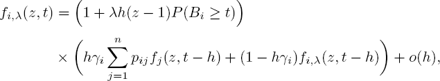
THEOREM 5.1.– The joint transform f (s, z, t) satisfies the following PDE with boundary condition f (0, 1, t) = 1:
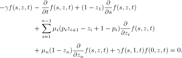
PROOF.– We exploit the fact that {(Λ(t),X1(t),...,Xn(t)), t ≥ 0} is a Markov process. At some given time t, let us assume Xi (t) = ki for each i, and Λ (t) = λ. In [t, t + h),h ↓ 0, three things can occur: a customer completes phase i of its service at rate kiμi; a customer arrives at rate λ; the arrival parameter resamples at rate γ. Hence

Straightforward calculations now yield
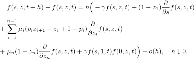
Dividing by h and letting h ↓ 0 leads to the PDE [5.1].
Let the vector (Λ, X1,..., Xn) be the steady-state version of the time-dependent (Λ(t),X1(t) ,..., Xn(t)) and write f(s,z) := ![]() . The following corollary then immediately follows from Theorem 5.1.
. The following corollary then immediately follows from Theorem 5.1.
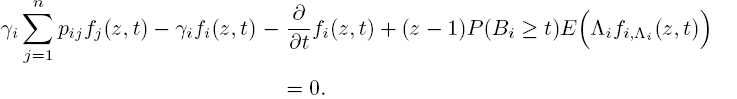
COROLLARY 5.1.-
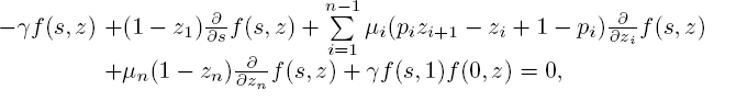
with f (0,1) = 1.
Solving either of the equations [5.1] or [5.2] is no easy task. Both are in the class of semilinear first-order PDEs. The usual solution approach would therefore be the method of characteristics (see, for example, (Salih 2016)). However, the appearance of f (0, z, t) (and f (0, z)) also makes it a delay equation. Hence, we cannot use standard techniques to compute an exact solution.
Numerical approaches for solving partial delay differential equations have been considered, though most often for very specific types. Finding a suitable method seems hard, and it remains a problem to solve [5.1] and [5.2] either analytically or numerically.
NOTE 5.1.- Taking z1 = ... = zn = 1, equation [5.1] becomes ![]() = 0 Therefore, the marginal transform
= 0 Therefore, the marginal transform ![]() is independent of t − and hence so is the distribution ofΛ(t). For each point in time t, Λ(t) has distribution GΛ. Of course, considering Λ(t) is still valuable for analyzing correlations with Λ(t′) or Xi(t′) for some t ′ ∈ IR. From now on, when we are not concerned with such correlations, we simply write Λ instead of Λ(t).
is independent of t − and hence so is the distribution ofΛ(t). For each point in time t, Λ(t) has distribution GΛ. Of course, considering Λ(t) is still valuable for analyzing correlations with Λ(t′) or Xi(t′) for some t ′ ∈ IR. From now on, when we are not concerned with such correlations, we simply write Λ instead of Λ(t).
NOTE 5.2.- Taking s = 0 in [5.2] yields
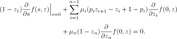
Although this equality does not seem to have a direct interpretation, it does when we take z1 = ... = zn and subsequently take z = 1. We then get
with S representing the sojourn time, one could compare this to Little’s formula λ = E(X)/E(S) for any standard queue. Since the sojourn time equals the service time in our infinite-server setting, ![]() is the rate at which a service is completed. Note that
is the rate at which a service is completed. Note that

so that Little’s formula indeed holds with λ replaced by E(Λ).
5.2.2. Calculating moments
One important feature of a generating function or Laplace–Stieltjes transform is the ability to quickly extract any moments for the corresponding random variable. In this section, we show that the PDE [5.1] provides enough information to do just that. More specifically, it allows us to calculate any moment of (Λ (t), X1(t), ... ,Xn (t)) by solving a recursion.
Let k denote the vector (k1,..., kn)T . If we would have an expressionforf (s, z, t), then the (l, k)th moment could be calculated by

NOTE 5.3.– Formally the moment should be defined as ![]() rather than
rather than ![]() . However, the former can easily be obtained from the latter.
. However, the former can easily be obtained from the latter.
Applying these same differentiations to PDE [5.1] yields, with ![]() denoting the mth derivative w.r.t. x:
denoting the mth derivative w.r.t. x:

Now define E (l, k1 ,..., kn, t) := ![]() as a shorthand notation for the joint moment. When we take s = 0, z = 1and use [5.4], we obtain
as a shorthand notation for the joint moment. When we take s = 0, z = 1and use [5.4], we obtain

our aim is to show that the recursive formula [5.5] allows one to iteratively compute all moments of(Λ (t), X1(t) ,..., Xn(t)), assuming all moments of GΛ are known. Let us first make the assumption that the system is empty at t = 0. If not, we split Xj(t) into the customers who arrived before or after t = 0. The contribution to Xj(t) of arrivals before time 0 can be calculated if we know (X1(0), ..., Xn(0)),by finding the probabilities pij(t) that a customer who was in phase i at time 0 is in phase j at time t. Conditioning on the case that it takes exactly u time to move from phase i to phase j,
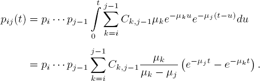
Here, ![]() and
and ![]() is the density of a hypoexponential distribution (see (Ross 2010, p. 310)). Recall that a hypoexponential random variable is a sum of independent exponentials (in our case j − i exponentials with rates μi,...,μj−1, respectively). It can also be seen as a Coxian random variable for which all continuation probabilities pk = 1.
is the density of a hypoexponential distribution (see (Ross 2010, p. 310)). Recall that a hypoexponential random variable is a sum of independent exponentials (in our case j − i exponentials with rates μi,...,μj−1, respectively). It can also be seen as a Coxian random variable for which all continuation probabilities pk = 1.
Let Yij (t) ~ Bernoulli(pij (t)) for i ≤ j, and let Yij,m (t), m = 1, 2,... be i.i.d. copies of Yij (t). Then the fraction of customers from Xj (t) that arrived before t = 0 equals

Now that we have found the fraction of customers from Xj (t) that arrived before t = 0, let us assume for the remainder of the section that the system is empty at time 0.
THEOREM 5.2.– All moments of (Λ (t), X1 (t),...,Xn (t)) can be computed using [5.5], and have the form
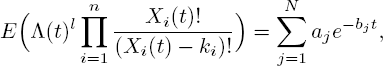
for some constants a1 ,..., aN and non-negative constants N, b1 ,..., bN.
PROOF.– We provide an inductive argument. In remark 5.1, we have seen that the distribution of Λ (t) is independent of t. In particular, E(Λl (t)) is constant in t, so the statement is true when taking k1 = ... = kn = 0.
Let us take a look at the structure of the recursion [5.5]. The derivative of the moment with (l, k1 ,..., kn) equals a linear function consisting of four unknown components: (1) the moment itself, (2) the same moment with k1 − 1 and l + 1, (3) the same moment with kj − 1 and kj− 1 + 1 for some j = 1, ..., n − 1, and (4) the same moment with l = 0.
Let ![]() . We have shown above that the statement is true for
. We have shown above that the statement is true for ![]() . The inductive step is split into two parts. First, assume we know all moments of order (l, K − 1) and we want to calculate all moments of order (0, K). Note that when substituting (0, K), component 4 coincides with component 1, and component 2 is known by assumption. From E (1, K − 1, 0,..., 0, t), we can calculate an arbitrary moment E (0, k1,..., kn, t) oforder(0,K) with the following scheme:
. The inductive step is split into two parts. First, assume we know all moments of order (l, K − 1) and we want to calculate all moments of order (0, K). Note that when substituting (0, K), component 4 coincides with component 1, and component 2 is known by assumption. From E (1, K − 1, 0,..., 0, t), we can calculate an arbitrary moment E (0, k1,..., kn, t) oforder(0,K) with the following scheme:

Note that for each arrow, a differential equation needs to be solved.
For the second part of the induction step, we assume that all moments of order (l′, K − 1) and (0, K) are known, and want to calculate all moments of order (l, K). In this case, both components 2 and 4 are known by assumption. The arbitrary moment E (l, k1,..., kn, t) of order (l, K) can now be calculated using the following scheme:

Combining both schemes, we can iteratively find an expression for any moment E (l, k1 ,..., kn, t). All that remains is to show that the moments take the form of [5.6]. This will be done by induction on the number of iterations.
Assume all moments calculated thus far take the form of [5.6]. Note that each iteration requires the differential equation [5.5] to be solved. This differential equation has the form
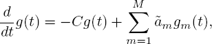
where C, M, ![]() are constants of which C, M are non-negative and gm (t) are known functions from previous iterations. Since the gm (t) have the required form by assumption, it holds that
are constants of which C, M are non-negative and gm (t) are known functions from previous iterations. Since the gm (t) have the required form by assumption, it holds that
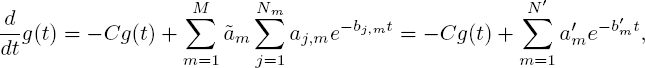
for some constants ![]() of which
of which ![]() are non-negative. Solving this differential equation quickly leads to the result of the theorem.□
are non-negative. Solving this differential equation quickly leads to the result of the theorem.□
NOTE 5.4.- It is an interesting question how many different terms a moment consists of, given its order (l, k1, ..., kn). In other words, how large is N in [5.6]? To answer this, note that when wesolve the differential equation [5.7] the only exponent we have not seen in previous iterations is −Ct. So N is at most the number of possible values of C. Checking with [5.5], we conclude that ![]() .
.
In terms of computational complexity, observe that [5.5] has O(n) terms, each one consisting of one momert. Since a moment has ![]() terms, one iteration requires
terms, one iteration requires ![]() operations. Note also that we need one iteration for each moment of lesser order. Therefore, the calculation of a moment of order (l, k1 ,..., kn) requires
operations. Note also that we need one iteration for each moment of lesser order. Therefore, the calculation of a moment of order (l, k1 ,..., kn) requires ![]() operations.
operations.
Now that we have seen that all moments can be retrieved, and which form they have, let us calculate some of these moments. This gives an idea how the system behaves in general and presents a quantitative way to compare our queue to other models.
One can check that expressions from higher moments become very large and complicated, requiring much computational effort and making analysis difficult. However, for some lower moments and special cases, we can derive “nicer” expressions. This enables us to give intuitive explanations and perform proper analyses on the formulas we used.
We start with an expression for the mean number of customers.
THEOREM 5.3.– Let ![]() . Given that the system is empty at t = θ, the mean number of customers in phase j at time t equals
. Given that the system is empty at t = θ, the mean number of customers in phase j at time t equals
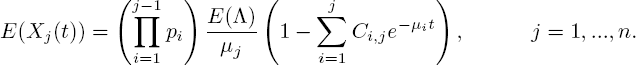
PROOF.– Let us first consider the case j = 1. Substituting k1 = 1 and l = k2 = ... = kn = 0 gives the differential equation
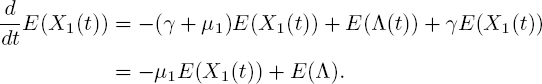
With E (X1(0)) = 0, its solution is
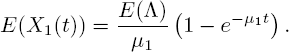
Therefore, [5.8] holds for j = 1.
Now let j ∈ {2, ..., n}. The differential equation corresponding to kj = 1 is
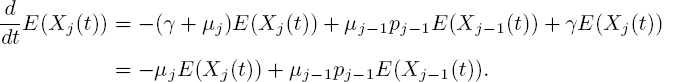
To show that [5.8] is indeed a solution to this equation, we differentiate [5.8] and rearrange terms, using that ![]()

To verify that solution [5.8] to differential equation [5.10] is the desired solution, we need to show that [5.8] satisfies the boundary condition E (Xj(0)) = 0. So what remains is to check that ![]() Ci,j = 1. We can do this by observing that
Ci,j = 1. We can do this by observing that
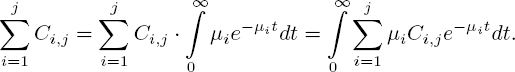
As has been proven (Ross 2010, pp. 309-310), the integrand is a density function of a random variable on [0, ∞). It follows that![]() Ci,j = 1, which concludes the proof.
Ci,j = 1, which concludes the proof.
For further moments, it is necessary to find E (Λ (t)X1(t)) first. So with l = k1 = 1 and k2 = ... = kn = 0, [5.5] gives
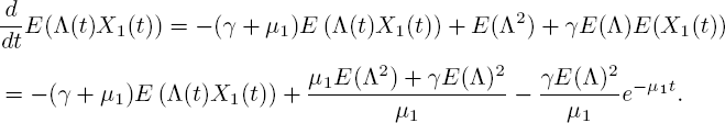
Here, we used the E(X1(t)) we found in [5.9]. Combined with the boundary condition E(Λ (0)X1(0)) = 0, the solution equals

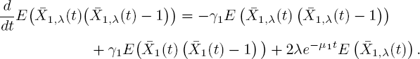
Next, we use the same trick for E (X1(t)(X1(t) − 1)). The differential equation for k1 = 2 and l = k2 = ... = kn = 0 is
with E (X1 (0) (X1 (0) − 1)) = 0. This has the solution
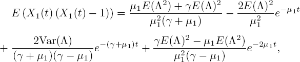
and it follows that
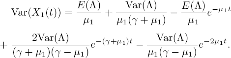
It is easily verified that γ = μ1 is not a singularity.
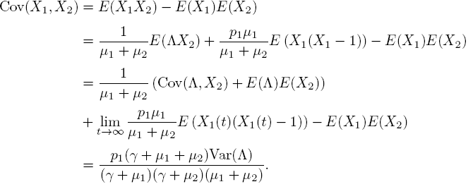
The correlation between Λ(t) and X1(t) follows from [5.11] and [5.13]
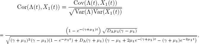
where ![]() is the dispersion index. Interestingly, the arrival process manifests itself only through DΛ. The positive correlation that the formula indicates makes sense, since correlation between Λ(t) and X1(t) can only occur when Λ (t) shows variability.
is the dispersion index. Interestingly, the arrival process manifests itself only through DΛ. The positive correlation that the formula indicates makes sense, since correlation between Λ(t) and X1(t) can only occur when Λ (t) shows variability.
As it is visible in Figure 5.1, there appears to be a time where the correlation is maximal. This will be the time tmax that enough customers could have arrived to show correlation, buta large fraction of X1 (tmax) still originates from the current Λ (and not from previous ones).
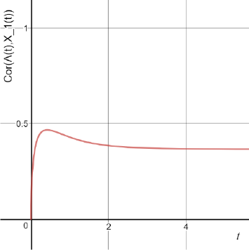
Figure 5.1. Cor(Λ(t), X1 (t)) for μ1 = 1, γ = 2 and DΛ = 2. For a color version of this figure, see www.iste.co.uk/anisimov/queueing1.zip
5.2.3. Steady state
In this section, we consider the steady-state behavior of the infinite-server queue, again focusing on a recursion for the joint moments of arrival rate and numbers of customers in phases 1,....,n.Let![]() Letting t →∞in [5.5] yields the following steady-state recursion:
Letting t →∞in [5.5] yields the following steady-state recursion:

Note that an iteration step only requires some basic operations, whereas in the transient case each iteration required a differential equation to be solved.
Let us find the steady-state mean number of customers in phase j. Taking kj = 1 (and everything else 0) yields

This simple recursion results in

which of course we could also have found from [5.8] letting t → ∞.
NOTE 5.5.- Recall that the mean number of customers in an ordinary M/M/∞- queue is ![]() , the arrival rate divided by the departure rate. Formula [5.16] represents something similar: the expected arrival rate over the departure rate in phase j.To see this, note that with
, the arrival rate divided by the departure rate. Formula [5.16] represents something similar: the expected arrival rate over the departure rate in phase j.To see this, note that with ![]() being the probability that a customer reaches phase j,
being the probability that a customer reaches phase j, ![]() is the expected arrival rate of phase j.
is the expected arrival rate of phase j.
With the steady-state mean at hand, formula [5.8] has a nice interpretation. We consider the steady-state number of customers who are in phase j (given in [5.16]), and distinguish the fraction that has been in the system for at least t time, and the fraction that has not. Where the steady-state mean consists of both fractions, the transient mean [5.8] only consists of the second (assuming an empty system at time 0). Now note that a customer in phase j has gone through j exponential phases (1 up to j − 1 completely and the past part of an exponential phase j). So the second fraction is proportional to the probability that j exponential phases are traversed before time t. According to formula [5.8], this probability should be ![]() . Indeed, this is precisely the distribution function of a hypoexponential random variable.
. Indeed, this is precisely the distribution function of a hypoexponential random variable.
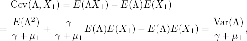
Another quantity that is greatly simplified by considering steady state is Cov(Λ, Xj). For this, we take l = kj = 1 in [5.15] and find
such that
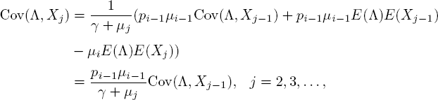
returns a simple recursion. We also observe that
hence the solution is

This formula also provides an interesting interpretation. Recall that ![]() is the probability that an exponential time with rate μ is shorter than an exponential time with rate γ. Therefore,
is the probability that an exponential time with rate μ is shorter than an exponential time with rate γ. Therefore, ![]() is the probability that a customer traverses j − 1 service phases before the arrival parameter resamples. The appearance of this probability is intuitive, since the current Λ can only influence the current Xj if customers generated from this Λ arrive in phase j before a new Λ is drawn.
is the probability that a customer traverses j − 1 service phases before the arrival parameter resamples. The appearance of this probability is intuitive, since the current Λ can only influence the current Xj if customers generated from this Λ arrive in phase j before a new Λ is drawn.
Next, we check the variance of the number of customers in phase 2. To do this, we substitute k2 = 2 in[5.15]. In the calculation, we also use[5.17]forj = 2 and [5.12] for t → ∞

so that
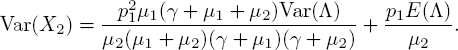
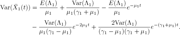
Let us state the variance of the steady-state number of customers in phase 1:
(t → ∞ in [5.13]). It is easy to check that E(X2) = E (X1) and Var (X2) ≤ Var (X1) when p1 = 1 and μ1 = μ2 = μ. A numerical result shown next will elaborate on this last remark.
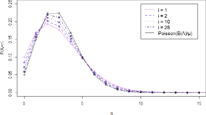
Figure 5.2. Estimated distribution of Xi for several phases i, with Λ ~ U (0, 6) and γ = μ = 1. For a color version of this figure, seewww.iste.co.uk/anisimov/queueing1.zip
Figure 5.2 visualizes the results of a simulation, where the service time distribution is taken to be Erlang with a large number of phases. The results give an impression of how the distribution of Xi evolves for growing i. Each line represents the distribution of the number of customers in the service phase corresponding to its color. Clearly, higher phases show less variability (while the mean remains unchanged due to p1 = ... = pn = 1 and μ1 = ... = μn = μ, see [5.16]). It should also be noted that the distribution of the number of customers in phase i tends to a Poisson distribution for large i. This can be explained by the fact that consecutive customers spread out over different phases. The effect of the mixed arrival rate then slowly decays for increasing phase numbers, and eventually the stream of customers from phase i − 1 to i barely differs from a Poisson process. Therefore, it is intuitive that Xi converges to a Poisson random variable with mean ![]() .
.
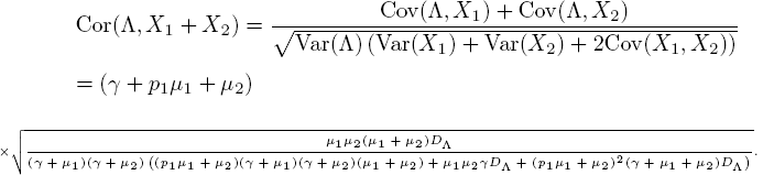
Using the variance of X2, we now calculate the correlation
In the special case that μ1 = μ2 = μ, we have
To compare, we let t → ∞ in [5.14] to get Cor(Λ, X1):

In cases where the service rates are equal (i.e. μ1 = μ2 = μ), it holds that
because p1 ≤ 1. An immediate consequence from this calculation is that Cor(Λ ,X1) ≥ Cor(Λ, X2) when the service rates are equal. This is not surprising, since customers “generated” by the current arrival rate Λ immediately arrive in phase 1, but take some time before entering phase 2 (if they remain in the system after phase 1). So earlier phases have a more direct connection with the current arrival rate.
The inequality does not necessarily hold for different service rates. To see this, note that when p1 is high and μ1 is high compared to μ2 and γ, customers spend more time in phase 2 than in phase 1 before the arrival parameter resamples.
Let us finally take a look at X1 + X2, which is the total number of customers for n = 2. Its mean and variance can easily be computed, but its correlation with Λ is less straightforward. To find it, we first have to determine Cov(X1, X2). This is done by taking k1 = k2 = 1 in [5.15], and using the moments given in [5.17], [5.12] and [5.16]:
Then with [5.17], [5.13], [5.18] and [5.21], we find
Note that when p1 = 0, customers never reach phase 2. It is easy to check that in that case, it indeed holds that Cor(Λ, X1 + X2) = Cor(Λ, X1).
5.2.4. MΛ/M/∞
In this section, we give a few results for the special Coxian case where the service time distribution is exponential with parameter μ. An easy way to recover the main results is by observing that this service time distribution can be obtained by taking p1 = ... = pn−1 = 0 and μ1 = μ. We then find
as the PDE for the joint transform of(Λ, X) and
as the recursion for moments. The observant reader may have noticed that all pi, i > 1 are irrelevant when p1 = 0, because customers can only be in phase 1. The extended assumption is made to more easily copy results from Coxian service times.
If Λ ~ exp(θ), we can derive an expression for the form of any moment.
THEOREM 5.4.– Let Λ ~ exp (θ). Then the recursion [5.24] has solution

where c0 (l, k) = 1, ck(l,k) = ![]() and Cj (l, k) satisfies the recursion
and Cj (l, k) satisfies the recursion
For a proof by induction, we refer to (van Kreveld 2018). Let us here only check that [5.26] has a solution. The key observation is that the second argument is lowered in each step of the recursion. Note that when we express cj (l, k) into coefficients of the form cj′(l′, k − 1) by using [5.26], we have either j′ = 0, j′ ∈ {1,..., k − 2} or j′ = k − 1. In the first and third case, the value is given, and in the second case we can use [5.26] again. Repeating this procedure k − 1 times leaves us with only unknown terms with k = 1. Since j ≤ k, the remaining coefficients are of the form c0(l′, 1) and c1 (l′, 1). These are both known, so the recursion ends after k − 1 steps.
As we have seen, the mean number of customers is similar in M/M/∞ and MΛ/M/∞, the only difference being that the fixed arrival rate λ is replaced by the expected arrival rate E(Λ). Mixing turns out to have a larger effect on the variance. Without mixing, the variance of X is equal to the mean, but our model has
as a consequence of [5.13] by taking μ1 = μ and t → ∞. The first term is the variancewithoutmixing, and the second is caused by the variability of the arrival rate. It is therefore no surprise that the second term is linear in Var(Λ).
Heemskerk et al. (2017) provide another interesting comparison for the variance. They consider the same model, the only difference being deterministic resample intervals with common length Δ. For the variance of the number of customers, Heemskerk et al. (2017) obtain
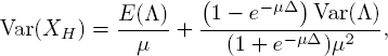
where XH denotes the steady-state number of customers in this model.
For a fair comparison between [5.27] and [5.28], we take ![]() , such that the mean resample interval lengths of both models agree. It clearly holds that Var (X) > Var (XH) if and only if
, such that the mean resample interval lengths of both models agree. It clearly holds that Var (X) > Var (XH) if and only if ![]() . Hence
. Hence
One might expect that randomness of resample interval lengths leads to more variability in X. Surprisingly, this result shows that is not always true.
For a good image of the distribution of X, we use a simple simulation, ofwhich the details can be found in (van Kreveld 2018). Keeping track of the number of customers in the MΛ/M/∞, the results for simulating up to t = 106 can be seen in Figure 5.3.
Note that with Λ ~ U (0, 6) and γ = μ = 1, we have E (X) = 3 and Var (X) = 4.5. On a single run, the simulation rarely returns an error of more than 0.01 foreach quantity.
To investigate the role of the resample rate γ for the distribution of X, we make a plot for several values of γ (Figure 5.4). Although the mean number of customers is the same for each value, we see that the variance decreases when γ increases. This observation is in line with formula [5.27].
A particularly noteworthy case is γ → ∞. It then follows from [5.27] that Var (X) → E (X). In fact, looking at Figure 5.4 we may even suspect that X converges to a Poisson random variable. This is intuitively explained as follows: when the number of resamples between two arrivals grows to infinity, the arrival process behaves like a Poisson process with rate E (Λ).
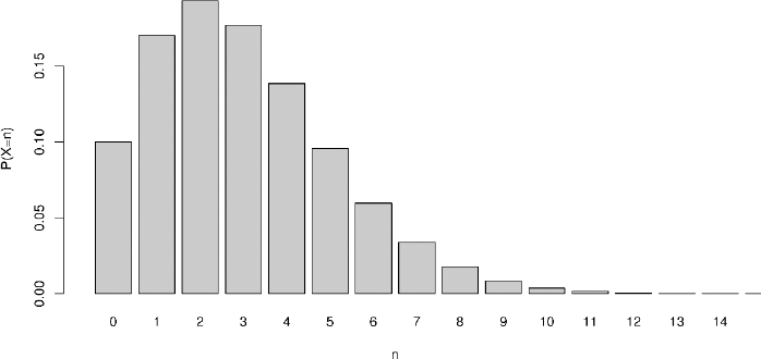
Figure 5.3.Histogram estimating the distribution of X, with Λ ~ U (0, 6) and γ = μ = 1
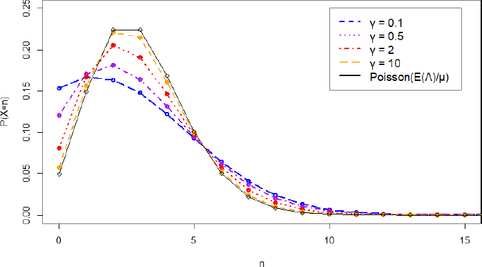
Figure 5.4. Estimated distribution of X for different values of γ, with Λ ~ U(0, 6) and μ = 1. For a color version ofthis figure, see www.iste.co.uk/anisimov/queueing1.zip
The last quantity we analyze regarding the steady-state vector (Λ, X) is the correlation between Λ and X. It is given by [5.20], replacing μ1 by μ as is explained at the start of this section.

Figure 5.5.Cor(X,Λ) for DΛ = 1 andγ = 0.5. For a color version of this figure, see www.iste.co.uk/anisimov/queueing1.zip
In Figure 5.5, we see that the correlation is low both when the service rate is very low or very high. This can be explained as follows: for the correlation to be high, on the one hand the service rate should not be too high since we want customers generated by the current Λ to stay as long as possible. On the other hand, the service rate should not be so low that “old” customers from previously sampled Λ stay in the system for too long. The correlation turns out to be maximal for ![]() attaining the value
attaining the value

Notice its dependence only on DΛγ.
We conclude this section with a brief discussion of scaling limits. We consider a scaling of the arrival rate Λ (t) with a factor N together with a scaling of the resample rate γ with factor Nα. The value of α determines which rate speeds up faster. If α > 1, the arrival rate changes very often, while if α < 1, the arrival rate rarely changes relative to the number of arrivals. We check the behavior of the MΛ/M/∞ under this scaling and discuss the effect of the value of α. We follow the idea of Heemskerk et al. (2017, pp. 8-12), in which they consider a model with the arrival parameter resampling aftera fixed time Δ.
Let X(N) be the steady-state number of customers under the corresponding scaling. Then we easily see that
and from [5.27] that
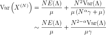
when N tends to infinity. This can be compared to the asymptotic variance of Heemskerk et al. (2017). Denoting by ![]() the number of customers in their model, they find
the number of customers in their model, they find

In both models, the variance increases as the average length of a resample interval ![]() increases. However, for the variances to be equal, it must be that
increases. However, for the variances to be equal, it must be that ![]() In other words, our more random model needs twice as many resamples to obtain the same asymptotic variance.
In other words, our more random model needs twice as many resamples to obtain the same asymptotic variance.
From [5.30], the limiting behavior of the variance is

Let β = max {1, 2 − α}. The asymptotic behavior suggests the following central limit theorem.
CONJECTURE 5.1.- Assume all moments of Λ are finite. If N → ∞, then
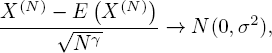
with ![]() .
.
The statement of the conjecture is very similar to theorem 2.1 from Heemskerk et al. (2017). However, in the proof they use they remark that the resample interval lengths are constant. This property is critical in the proof, making it hard to prove our conjecture using the same idea. Nonetheless, it is expected that the statement holds in our model as well.
5.3. Mixing in Markov-modulated infinite-server queues
In this section, we consider a Markov-modulated infinite-server queue. The Markov background process moves through a finite number of states N = {1, ..., n}; be aware that this n has nothing to do with the number of phases in the Coxian distribution considered in the previous section. While the process is in state i ∈ N, it takes an exponential amount of time with parameter γi before the state changes. When it does, it has probability pij to move to state j. Of course, pij ≥ 0 for each (i, j) ∈ N × N and![]() pij = 1 for each i ∈ N. Note that the Markov process behaves independently of the queue and acts only as a generator.
pij = 1 for each i ∈ N. Note that the Markov process behaves independently of the queue and acts only as a generator.
In state i ∈ N, customers arrive according to a Poisson process with random rate Λi, drawn according to a probability density function ![]() This rate is drawn at the start of the current state, and resampled once the state changes again; the arrival parameter also resamples if the Markov process moves to the same state. Bi is the service time of a customer arriving when the background process is in state i.
This rate is drawn at the start of the current state, and resampled once the state changes again; the arrival parameter also resamples if the Markov process moves to the same state. Bi is the service time of a customer arriving when the background process is in state i.
The difference with other Markov-modulated queueing models lies within the random parameter Λi. In standard Markov-modulated queues, the interarrival times have a fixed distribution depending on i; most commonly an exponential distribution with rate λi. In our case, when we apply mixing, the interarrival time distribution is exponential with a random rate Λi.
NOTE 5.6.– Observe that the workload of a customer is only dependent on the state in which it enters the system, not necessarily on the current state. In case the state of the background process changes before the customer ends its service, service continues with the service time drawn from the previous state.
In this section, we present the idea of Blom et al. (2014) applied to our concept of mixing the arrival parameter. First, we develop a differential equation that shows similarities with [5.1] from the MΛ/Coxn/∞ queue. Like in the previous section, we indicate how this differential equation can be used to obtain queue length moments.
5.3.1. The differential equation
We follow a similar approach as in Blom et al. (2014, section 3). Let S(t) ∈ N be the state of the Markovian background process at time t. Also, let ![]() be the number of customers at time t given X (0) = 0, S (0) = i and Λ (0) = λ. Assuming an empty system at time zero is, for the same reason as in section 5.2.2, not very restrictive. Say for example that there are m customers at time zero. Each of those can be characterized by the state it arrived in and its residual service time. With this information, we can calculate the probabilities q1, ..., qm that the corresponding customer is still in the system at time t. Let Zj(t) ~ Bernoulli(qj) for j = 1,..., m. Then the total number of customers at time t equals
be the number of customers at time t given X (0) = 0, S (0) = i and Λ (0) = λ. Assuming an empty system at time zero is, for the same reason as in section 5.2.2, not very restrictive. Say for example that there are m customers at time zero. Each of those can be characterized by the state it arrived in and its residual service time. With this information, we can calculate the probabilities q1, ..., qm that the corresponding customer is still in the system at time t. Let Zj(t) ~ Bernoulli(qj) for j = 1,..., m. Then the total number of customers at time t equals ![]()
Consider the small time interval (0, h). Define fi,λ (z, t) := ![]() To remove the condition Λ (0) = λ, we define
To remove the condition Λ (0) = λ, we define ![]() as the number of customers at time t given X (0) = 0 and S (0) = i. Moreover, let fi (z,t) =
as the number of customers at time t given X (0) = 0 and S (0) = i. Moreover, let fi (z,t) = ![]() =
= ![]() be the corresponding generating function. It is easily seen that
be the corresponding generating function. It is easily seen that
which yields the differential equation

Removing the condition Λ(0) = λ then gives
This last formula has some interesting consequences. For example, by letting t → ∞, we find the steady-state formula
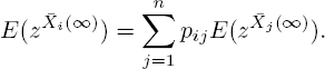
Note that after an infinite amount of time, the state of the background process at t = 0 should be irrelevant. Since ![]() . the above equality indeed holds.
. the above equality indeed holds.
Another interesting situation occurs when n = 1, so that the system is always in state 1. Note that this is a generalization of our previous ![]() model, the service times now having a fully general distribution. equation [5.35] in this case becomes
model, the service times now having a fully general distribution. equation [5.35] in this case becomes
Also taking the derivative with respect to z and taking z = 1 gives
which, with the condition that ![]() , yields
, yields

Taking B1 ~ exp(μ1) here, for example, gives
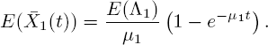
This formula of course agrees with formula [5.9] for the mean number of customers in phase 1 of the ![]() queue. When only considering customers in the first phase of a Coxian distribution, successive phases are irrelevant since there are infinitely many servers. Therefore, both models describe the MΛ/M/∞, and
queue. When only considering customers in the first phase of a Coxian distribution, successive phases are irrelevant since there are infinitely many servers. Therefore, both models describe the MΛ/M/∞, and ![]() when the background process has only one state and B1 ~ exp(μ1).
when the background process has only one state and B1 ~ exp(μ1).
5.3.2. Calculating moments
In the ![]() from section 5.2, we saw that despite being unable to find the generating function, we could use the differential equation to compute all moments. We will do the same here with the Markov-modulated queue, both with and without the initial condition on Λ(θ).
from section 5.2, we saw that despite being unable to find the generating function, we could use the differential equation to compute all moments. We will do the same here with the Markov-modulated queue, both with and without the initial condition on Λ(θ).
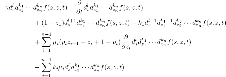
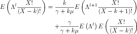
To obtain factorial moments, we take from [5.34] the kth derivative with respect to z in z = 1:

Doing the same with [5.35] gives

THEOREM 5.5.– All moments ![]() and
and ![]() can be iteratively computed for all k ∈ IN.
can be iteratively computed for all k ∈ IN.
PROOF.– Note that equation [5.38] can be seen as a system of linear differential equations
where
 is the n-dimensional vector consisting of
  up to
up to  ;
;- A is a matrix with entries aij = γipij for i ≠ j and aii = γi (pii − 1);
In the same way, [5.37] can be viewed as n separate differential equations

with

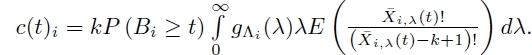
The main idea is that when we solve the equations in the right order, the c(t)i and c(λ,t)i are known from previous iterations. If these quantities are known, we can find any moment by solving equations [5.39] and [5.40] via ordinary differential equation methods.
We now proceed to show a sufficient calculation order to complete the proof, by induction. For k = 1, we have c(t)i = P(Bi ≥ t)E (Λi), enabling us to calculate ![]() for i = 1, ...,n with [5.39]. Now,
for i = 1, ...,n with [5.39]. Now, ![]()
![]() is known such that with [5.40] we can also find
is known such that with [5.40] we can also find ![]() .
.
Suppose we know all moments of order k − 1. Then c(t)i can be found by assumption, so we can solve the system [5.39] to find ![]() for i = 1, ..., n. With these quantities found and the induction hypothesis, note that now also c(λ, t)i are known. By solving [5.40], the proof is complete. □
for i = 1, ..., n. With these quantities found and the induction hypothesis, note that now also c(λ, t)i are known. By solving [5.40], the proof is complete. □
The next step is to calculate some specific moments with equations [5.37] and [5.38]. Specifying the service time distributions allows for expressions without integrals, so let us assume from now that Bi ~ exp(μi) for i = 1, ..., n. The exponential distribution is a natural choice and gives simple expressions.
Note that we already found ![]() for n = 1 in [5.36]. We proceed with finding the mean, conditioned on Λ(0) = λ, and the variance for n = 1. After that we move on to n = 2.
for n = 1 in [5.36]. We proceed with finding the mean, conditioned on Λ(0) = λ, and the variance for n = 1. After that we move on to n = 2.
With k = 1 and [5.36], differential equation [5.37] reads
One can easily check that, with boundary condition ![]() ,
,

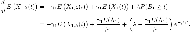
Some interpretation of this formula can be obtained when we write it as

We recognize the first term as the formula for ![]() . The second term is a non-negative number times the difference between the conditioned starting arrival parameter λ and its expectation E (Λ1). In other words, the difference in the mean queue size conditioned on Λ (0) = λ or Λ (0) = Λ1, is linear in λ − E(Λ1). It is evident that when t > 0,
. The second term is a non-negative number times the difference between the conditioned starting arrival parameter λ and its expectation E (Λ1). In other words, the difference in the mean queue size conditioned on Λ (0) = λ or Λ (0) = Λ1, is linear in λ − E(Λ1). It is evident that when t > 0, ![]() if and only if λ ≥ E(Λ1), with equality ifand only λ = E(Λ1).
if and only if λ ≥ E(Λ1), with equality ifand only λ = E(Λ1).
It also follows from [5.41] that the difference between ![]() is largest at
is largest at ![]() . The existence of a maximum is intuitive: at t = 0, the system still has to set up, and when t → ∞, the value of Λ (0) has become irrelevant. In both of these cases, it holds that
. The existence of a maximum is intuitive: at t = 0, the system still has to set up, and when t → ∞, the value of Λ (0) has become irrelevant. In both of these cases, it holds that ![]() .
.
Formula [5.41] also holds for the MΛ/COXn/∞ setting, in the sense that ![]() (see the end of section 5.3.1). The approach of section 5.2 does not enable us to find moments conditioned on Λ(0), so this is an interesting observation.
(see the end of section 5.3.1). The approach of section 5.2 does not enable us to find moments conditioned on Λ(0), so this is an interesting observation.
Moving on to moments of second order, we take k = 2 in [5.38] and find
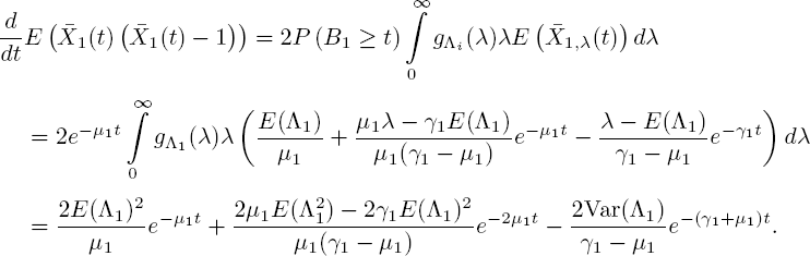
The only solution with ![]() is
is

and hence
This is in agreement with [5.13]; see also the end of section 5.3.1.
We proceed by studying the variance when the starting arrival rate is fixed, i.e. Λ(0) = λ. Using formula [5.38] for k = 2 yields
Observe that the latter two terms are known from [5.42] and [5.41], hence we have a solvable linear differential equation. As usual, we set the boundary condition at E(![]() ), leading to E(
), leading to E(![]() ) and subsequently to
) and subsequently to

Note here that the initial arrival intensity only appears as λ − E (Λ1), and that γ = μ1 and γ = 2μ1 are removable singularities.
So far, we have only obtained explicit expressions for moments in the Markov-modulated queue with the background process having only one state. In order to better analyze the effect of the background process on the queue, we now consider an example with n = 2. This should give an impression of the behavior of the Markov-modulated queue with multiple states.
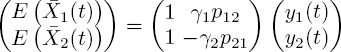
For n = 2, k = 1, [5.39] takes the form

since p11 − 1 = −p12 and p22 − 1 = −p21. We can solve this system with the eigenvalue method (see, for example, (Shen 2013)). Define π := γ1p12+γ2p21 as the sum of the state transition rates. It is easily seen that the eigenvectors of the system are ![]() and
and ![]() with eigenvalues 0 and -π, respectively. Therefore, the solution is
with eigenvalues 0 and -π, respectively. Therefore, the solution is
with

The latter is a pair of separate linear differential equations. Solving these, substituting in the above solution and again using the boundary condition ![]() , yields
, yields
Quantities in [5.45] that should be recognized are
 and
and  , the long-term fractions of finding the Markov process in states 1 and 2, respectively;
 , the mean number of customers when the Markov process is always in state i (i = 1, 2);
 , a non-negative quantity that increases whenever π or μi increases (i = 1, 2).
With these equations we can also find some other relevant quantities. For example, suppose that the state at time 0 is not known, but the background process is in steady state. Then ![]() and
and ![]() , so it follows that the mean number of customers at time t is
, so it follows that the mean number of customers at time t is
Another consequence of [5.45] is the steady-state mean
Keep in mind that there is no subscript needed, since in steady state it does not matter in which state we started. In the formula, we see the steady-state mean of each individual state, multiplied by the fraction that the corresponding state was active. The fact that the steady-state mean is just the sum of these parts underlines that customers from different states do not interfere with each other.
Let us now consider ![]() : the steady-state expected number of customers given the background process is in state 1. Before we can give an expression, we have to define
: the steady-state expected number of customers given the background process is in state 1. Before we can give an expression, we have to define ![]() as the portion of the current customers who arrived when the state was i. Distinction between
as the portion of the current customers who arrived when the state was i. Distinction between ![]() and
and ![]() is relevant because customers who arrived in a different state will have a different service rate. For instance, the first term of [5.47] is the mean number of customers with service rate μ1 .
is relevant because customers who arrived in a different state will have a different service rate. For instance, the first term of [5.47] is the mean number of customers with service rate μ1 .
Now define T1 as an arbitrary time in steady state when the background process moves from state 1 to state 2. Also, let T2→1 be the last time before T1 that the state changed from 2 to 1. We split ![]() into the customers who arrived before or after T2→1 , and then condition on the value of T1 − T2→1 . It holds that
into the customers who arrived before or after T2→1 , and then condition on the value of T1 − T2→1 . It holds that
Let T2 and T1→2 be the symmetric versions of T1 and T2→1. We then have

A useful observation here is that ![]() and
and ![]() , since in each case, both times represent a steady-state time at the end of a period of one state. As a result, we have a system of two linear equations. The solution is
, since in each case, both times represent a steady-state time at the end of a period of one state. As a result, we have a system of two linear equations. The solution is
Note the absence of E(Λ2) and μ2 caused by the fact that customers from different states do not influence each other.
Let TS = 1 be an arbitrary steady-state time with S(TS=1 ) = 1. We will show that ![]() . Note that we can view the Markov background process as a Poisson process with rate γ1p12, and we can view its events as periods where the state is 2. We assume those periods take 0 time, so that the rate at which an event happens is always γ1p12. A nice property of the Poisson process is that when we pick an arbitrary point in time (Ts=1 ), the amount of time since the last event is exponentially distributed with parameter γ1p12. The same holds for T1, so
. Note that we can view the Markov background process as a Poisson process with rate γ1p12, and we can view its events as periods where the state is 2. We assume those periods take 0 time, so that the rate at which an event happens is always γ1p12. A nice property of the Poisson process is that when we pick an arbitrary point in time (Ts=1 ), the amount of time since the last event is exponentially distributed with parameter γ1p12. The same holds for T1, so ![]() , hence in particular E
, hence in particular E![]()
![]() .
.
As a quick sanity check, we calculate E(![]() ), the steady-state mean number of customers who arrived when the background process was in state 1 (i.e. the customers who have service rate μ1). As mentioned, this should give the first term of [5.47]. The calculation below verifies this:
), the steady-state mean number of customers who arrived when the background process was in state 1 (i.e. the customers who have service rate μ1). As mentioned, this should give the first term of [5.47]. The calculation below verifies this:

For symmetry reasons, [5.48] can be transformed into

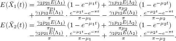
Now we are finally ready to find the mean total number of customers conditioned on the current state:
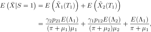
and analogously,
Given the complexity of calculations with two states, formulas for general n will be costly to derive analytically. However, if one assumes that the Markov process is in steady state at time 0, one can use a shortcut found by Blom et al. (2014) for the mean number of customers. It is based on the well-known rate-in = rate-out balance equation ![]() , being the steady-state probabilities for each state.
, being the steady-state probabilities for each state.
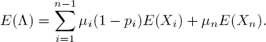
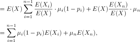
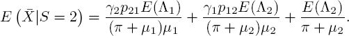
To find the mean number of customers in this case, we take k = 1 in [5.38], multiply by πi and sum over i. This results in
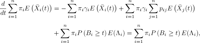
and hence
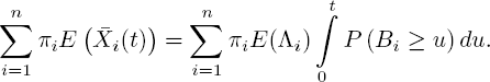
With relatively easy methods, we found a general formula for the mean. For instance, n = 2 and exponential service times yields [5.46], which was more difficult to find as we had to solve a system of differential equations. The disadvantage of the quicker method is that it gives no information about the case where the starting state S(0) is fixed.
5.4. Discussion and future work
We have considered two infinite-server queueing models with a mixed arrival process. For the MΛ/Coxn/∞ model with exponential resample times, we showed how to compute all joint moments of the arrival rate and the number of customers, both in transient and steady state. For a Markov-modulated queue with general service times, we gave a procedure to obtain all moments of the number of customers given the initial state and the initial arrival rate.
Since moments define a distribution, finding a way to compute them is a significant step toward finding the exact queue size distribution, even though we could not find a closed formula for all moments. Possible future research may include finding the exact distributions of the considered random variables. From our point of view, a way to do this is solving the PDE corresponding to that model.
In related papers about infinite-server queues, a considerable amount of work has been done regarding scaling limits and large deviation principles (Anderson et al. 2016; Blom et al. 2014; Heemskerk et al. 2017; Jansen et al. 2016). It is likely that similar results can be proven for our models (see Conjecture 5.1).
Finally, it would be interesting to study the M/M/∞ queue in which not the arrival rate but the service rate is described by a stochastic process. That infinite-server queue seems less amenable to a recursive approach.
5.5. References
Adan, I., Resing, J. (2015). Queueing systems [Online]. Available: http://www.win.tue.nl/~iadan/queueing.pdf.
Albrecher, H., Asmussen, S. (2006). Ruin probabilities and aggregate claims distributions for shot noise Cox processes. Scandinavian Actuarial Journal, 86–110.
Anderson, D., Blom, J., Mandjes, M., Thorsdottir, H., de Turck, K. (2016). A functional central limit theorem for a Markov-modulated infinite-server queue. Methodology and Computing in Applied Probability, 18, 153–168.
Anisimov, V. (2008). Switching Processes in Queueing Models. ISTE Ltd, London, and John Wiley & Sons, New York.
Asmussen, S. (2003). Applied Probability and Queues, 2nd ed. Springer-Verlag, New York.
Blom, J., Kella, O., Mandjes, M., Thorsdottir, H. (2014). Markov-modulated infinite-server queues with general service times. Queueing Systems, 76, 403–424.
Bühlmann, H. (1972). Ruinwahrscheinlichkeit bei erfahrungstarifiertem portefeuille. Bulletin de l’Association des Actuaires Suisses, 2, 131–140.
D’Auria, B. (2008). M/M/∞ queues in semi-Markovian random environment. Queueing Systems, 58, 221–237.
Daw, A., Pender, J. (2018). Queues driven by Hawkes processes. Stochastic Systems, 8, 192–229.
Eick, S., Massey, W., Whitt, W. (1993). The physics of the Mt/G/∞ queue. Management Science, 39, 241–252.
Heemskerk, M., van Leeuwaarden, J., Mandjes, M. (2017). Scaling limits for infinite-server systems in a random environment. Stochastic Systems, 7, 1–31.
Jansen, H.M., Mandjes, M.R.H., De Turck, K., Wittevrongel, S. (2016). A large deviations principle for infinite-server queues in a random environment. Queueing Systems, 82, 199–235.
Jongbloed, G., Koole, G. (2001). Managing uncertainty in call centres using Poisson mixtures. Applied Stochastic Models in Business and Industry, 17, 307–318.
Klaasse, B. (2017). Queuing and insurance risk models with mixing dependencies. Report, Eindhoven University of Technology.
Koops, D., Boxma, O., Mandjes, M. (2017). Networks of ./G/∞ queues with shot-noise driven arrival intensities. Queueing Systems, 86, 301–325.
Koops, D., Saxena, M., Boxma, O., Mandjes, M. (2018). Infinite-server queues with Hawkes input. Journal of Applied Probability, 55, 920–943.
van Kreveld, L.R. (2018). Parameter mixing in infinite server queues. MSc Thesis, University of Utrecht.
Neuts, M.F. (1981). Matrix-Geometric Solutions in Stochastic Models. Johns Hopkins University Press, Baltimore.
Neuts, M.F. (1989). Structured Stochastic Matrices of M/G/1 Type and their Applications. Marcel Dekker, New York.
O’Cinneide, C.A., Purdue, P. (1986). The M/M/∞ queue in a random environment. Journal of Applied Probability, 23, 175–184.
Raaijmakers, Y., Albrecher, H., Boxma, O. (2019). The single server queue with mixing dependencies. Methodology and Computing in Applied Probability, 21(82), forthcoming.
Ross, S. M. (2010). Introduction to Probability Models, 10th edition. Elsevier, New York.
Salih, A. (2016). Method of Characteristics. Indian Institute of Space Science and Technology, Thiruvananthapuram.
Shen, W. (2013). Introduction to ordinary and partial differential equations [Online]. Available: https://www.math.psu.edu/shen_w/LNDE.pdf