
7
Diffusion and Gaussian Limits for Multichannel Queueing Networks
Eugene LEBEDEV and Hanna LIVINSKA
National Taras Shevchenko University, Kiev, Ukraine
This chapter gives some results in diffusion and Gaussian approximation of multichannel queueing networks under heavy traffic conditions. Input flow of calls has a complicated structure. Moreover, its rate is allowed to be dependent on time. A local approach is used for the diffusion approximation of service process in multichannel networks with input flows of clearly defined structure. This approach enables us to prove limit theorems and establish convergence to a diffusion process with local characteristics, which can be specified explicitly via the network parameters. If there are no restrictions on the structure of the input flow, then the analysis procedure of a service process in multichannel networks changes. In this case, the limit process is described as a multidimensional Gaussian process. Proofs of the corresponding limit theorems are based on functional limit theorems for input flows as well as on the characteristic functions method. Often, the limit process turns out to be a Gaussian diffusion process. However, in this chapter, we mention conditions when the limit Gaussian process loses Markov property and it is not a diffusion process.
7.1. Introduction
In recent years, network research has acquired new practical importance as a primary tool for studying, designing and optimizing real-world systems with interconnected components. Queueing networks provide for them simple but extremely useful representation. The structure of such networks is determined by the probabilistic characteristics of the input flows and data processing algorithms. It is necessary to find their characteristics, optimize them and develop the corresponding control algorithms. Typically, the information processing in queueing networks is described by multidimensional vectors with interconnected entries, and the complex system of stochastic relations that define the process.
The main approach to the investigation of queueing networks is based upon the direct method of finding expressions for the network state probabilities. It allows us to find the exact solution for multiplicative or, as they are often called, locally balanced networks, with their stationary probabilities having a multiplicative form (see, for example, (Gnedenko and Kovalenko 2013, p. 84)). An alternative approach is to use the method of the asymptotic analysis for investigating complex systems and networks.
By asymptotic methods in queueing theory, one usually means the directions of investigations with their main objective to study complex multidimensional service processes using their approximation by processes with simpler structure. There are different versions of the limit conditions under consideration: extremely large interval of observations, small rate of service, increasing rate of input flows of calls, etc.
One of the first works in this direction is of Prokhorov (1956), where a Wiener process appears as an approximative process.
Diffusion approximation (DA) is a technique where a complicated and analytically intractable stochastic process is replaced by an appropriate diffusion process. A diffusion process is a Markov process having continuous sample paths. Diffusion processes considerably have an analytical structure and are, therefore, more mathematically tractable than the original process with which the user starts. Different approaches to DA of stochastic processes are elaborated. The traditional procedure for proving convergence of the sequence of stochastic processes to a limit process is to prove convergence of characteristic functions of finite-dimensional distributions of the sequence to the corresponding characteristic functions of the limit process. An essential fault of this procedure is that deriving characteristic functions of finite-dimensional distributions involves considerable technical difficulties and yields cumbersome expressions. Moreover, attempts in finding explicit form of finite-dimensional distributions of the limit process are not necessarily successful. In case of proving convergence to a diffusion process, these difficulties can be overcome by using the “local approach” to prove limit theorems (see, for example, (Borovkov 1980; Gikhman 1969)).
Convergence to diffusion processes using the local approach was first used by Bernstein (1934) and Khinchin (1936). Since general conditions for convergence to diffusion processes have been obtained in works of Gikhman, Skorokhod and Borovkov (Borovkov 1980; Gikhman 1969; Gikhman and Skorokhod 1982), the local approach became one of the main tools for strict mathematical justification of DA.
A large number of papers is devoted to the analysis of queueing models in heavy traffic conditions. There are several directions oriented to different classes of queueing models. Many authors deal with single-server nodes networks, renewal input process, independent service times and the routing processes that are independent of the current size of a queue or a workload process. For this case, the convergence of a normalized queue length or a workload process to a solution of a differential equation (fluid limits) or to a reflecting Brownian motion in a corresponding domain (Brownian approximation) is proved for a single-class network (Reiman 1984) and for various classes of multiclass networks (see surveys in (Williams 1996, 2016)).
Another direction is related to the analysis of Markov state-dependent queueing models. The method of analysis here is mainly based on a martingale technique and uses the continuous mapping theorems as well. This technique is used for the DA of some state-dependent networks in Basharin et al. (1989); Mandelbaum and Pats (1995) and Mandelbaum et al. (1998).
One more approach to study the fluid limits and the DA for some classes of state-dependent Markov queueing systems and networks is based on using the averaging principle (AP) and DA type results for so-called switching processes and for a special subclass of switching processes, recurrent processes of a semi-Markov type, introduced and developed in Anisimov (1995). Note that a switching process has the property that the character of its operation varies spontaneously (switches) at some epochs of time, which can be random functionals of the previous trajectory or possibly jumps of some random environment. Thus, this class serves as a convenient tool to describe wide classes of queueing models with state-dependent structure and operating in a random environment. The results of Anisimov (1995) are used and extended further to study AP and DA for rather general classes of queueing models of a switching structure (Anisimov 2002, 2008, 2010), etc.
Queueing Markov models whose evolution develops under the influence of random factors are studied in averaging and DA scheme in Korolyuk (1999). Such models (called Markov random evolution) are determined by two processes: a switched process describing the evolution of the system and a switching process describing changes of the random environment. Techniques for the analysis of random evolutions are based on the theory of singular perturbed reducibly invertible operators and on the martingale characterization of Markov stochastic processes. In Korolyuk et al. (2009), asymptotic average and DA schemes for semi-Markov queueing systems are studied by a random evolution approach and by using the compensating operator of the corresponding extended Markov renewal process.
We focus in this chapter on the analysis of the class of open queueing networks with an unlimited number of servers in each node (multichannel queueing networks). Since a direct analytical study of such models is not possible in most cases, we use methods of asymptotic analysis under heavy traffic conditions.
Queueing models with an infinite number of servers play an important role in the simulation of real systems. For example, similar models are considered: for the analytical modeling of information networks (Nazarov and Tuenbaeva 2009) and cellular communication networks (Massey and Whitt 1993, 1994); in the study of the parameters of the ionization track in tracking chambers (Dvurečenskij et al. 1981); in pharmacokinetics (Matis and Wehrly 1990); in economic models such as models in logistics, insurance, demography, etc.
Models with an infinite number of servers are widely covered in the scientific literature (see, for example, (Brian et al. 2009; Decreusefond and Moyal 2008; Moiseev and Nazarov 2015; Puhalskii and Reed 2008; Whitt 1982, 2016)). Asymptotic analysis of some multichannel queueing networks under condition of high-intensity input flow is considered in the papers by Moiseev and Nazarov (2016), of Nazarov and Moiseev (2014) and in the book by Moiseev and Nazarov (2015). The authors used their original methods: method of the first jump selecting and the method of multidimensional dynamic sifting.
In this chapter, we pay attention to studies of multichannel queueing networks under heavy traffic conditions. Input flow of calls can have a complicated enough structure, moreover, its rate is allowed to be dependent on time. Despite a great deal of recent works in the area of queueing networks, this class of models has not yielded to an exact analysis.
In the case when input flow has a clearly defined structure, it is efficient to use the local approach for DA of a service process in multichannel networks. This approach enables us to prove limit theorems and establish convergence to a diffusion process with its local characteristics, which can be specified explicitly via the network parameters. Throughout the chapter, convergence of processes implies convergence in the uniform topology. This is convenient because it yields convergence of the main functionals of stochastic processes paths. This feature allows us to formulate and solve problems connected with optimal choice of the network parameters.
If there are no restrictions on the structure of the input flow, then one should alter the analysis procedure of a service process in multichannel networks. In this case, it is suitable to describe the limit process as a multidimensional Gaussian process. Proofs of the corresponding limit theorems are based on functional limit theorems for input flows as well as on the characteristic functions method. Eventually, often the limit process turns out to be a Gaussian diffusion process. However, in the chapter we point out conditions when the limit Gaussian process loses Markov property and therefore is not a diffusion process.
This chapter is written based on authors’ publications in the scientific journals (Lebedev 2001, 2002b, 2003, 2017; Lebedev and Livinska 2017, 2018, 2019; Livinska and Lebedev 2016, 2018; Livinska 2016) and the conference papers (Lebedev 2002a; Livinska and Lebedev 2015). It is organized as follows:
In section 7.2, the main mathematical model is described in details.
Section 7.3 focuses on the local approach for proving limit theorems, and the main idea of the approach is described. In section 7.3.1, this technique is used for the DA of a service process of a multichannel network with recurrent input flow and exponential service.
In section 7.4, networks with a more complicated structure of input flow are studied. In section 7.4.1, for a [SM|M∣∞]r-network with input flow controlled by a semi-Markov process, DA is provided. Analysis of stationary regime for a network with generally distributed service times is given in section 7.4.2. In terms of these results, in section 7.4.3, it is established that the service process of the network operating in stationary regime converges to an Ornstein-Uhlenbeck process.
Section 7.5 is devoted to Gaussian approximation of multichannel networks of [G|M∣∞]r-type. In section 7.5.1, for such networks operating in a heavy traffic regime, an approximative Gaussian process is built, and its characteristics are specified via the network parameters. In section 7.5.2, the criterium of Markovian behavior is derived for multidimensional Gaussian processes. Moreover, it is found that the approximative Gaussian process from the previous section is a diffusion process. In section 7.5.3, for networks of [G|GI∣∞]r-type, convergence of the service process to a multidimensional Gaussian process is proved. In this case, under general assumptions, the limit process is a non-Markov one.
Section 7.6 provides Gaussian approximation for networks with a time-dependent input flow operating in a heavy traffic regime. In this, two cases with different starting loads are considered. For both cases, the Gaussian limit process is constructed. In the case of asymptotically large starting load considered in section 7.6.2, it is proved that the limit process is an Ornstein–Uhlenbeck process.
Section 7.7 concludes the chapter.
7.2. Model description and notation
Throughout the chapter, we will study similar networks. Therefore, in this section, our model for an open multichannel queueing network is described. More precisely, in the chapter, a family of networks is considered, each member of which may have a different collection of primitive processes. So, here we define: the structure of the network and routing algorithm, which are the same over all sections; the process of calls arrived from the outside, service time and initial conditions, which may be different in different sections.
Queueing networks under consideration consist of a fixed finite set r of service nodes (stations) through which calls (customers, jobs) are processed. A call visits nodes according to the routing algorithm below and receives service at each node visited. Each of the r nodes is a multichannel queueing system for serving calls. It means that each node has an infinite number of servers, thus, if a call arrives in such a system, then its service begins immediately and there is no queue of calls waiting for their service.
Routing algorithms through the network can be described as follows. Once the service of a call is completed in the ith node, the call is directed to the jth node with probability pij, or it leaves the network with probability ![]() . The r × r matrix
. The r × r matrix ![]() with entries pij is called the switching (routing) matrix of the network. An additional network node numbered by r +1 is interpreted as an “exit” from the network. To satisfy our open queueing network assumption, the matrix P is assumed to have spectral radius strictly less than one.
with entries pij is called the switching (routing) matrix of the network. An additional network node numbered by r +1 is interpreted as an “exit” from the network. To satisfy our open queueing network assumption, the matrix P is assumed to have spectral radius strictly less than one.
We assume that there is an r-dimensional external arrival process
such that for each i = 1, 2, ..., r ν(i)(t) is the number of calls arrived to the ith node from the outside of the network that have occurred by time t. Here and throughout the chapter, the superscript ′ is used to denote the operation of taking the transpose of a vector or matrix. For ν(t), we consider some options.
- – A recurrent flow of calls arrives to the ith node. Interarrival times are independent and identically distributed (i.i.d.) random variables with a distribution function Fi(t). We use notation [GI|.|∞]r for networks with this type of input flow.
- – A common input flow controlled by a semi-Markov process arrives from the outside to the network denoted by [SM|.|∞]r. The structure of such a flow is more complicated. A detailed description of this case is given in a relevant section.
- - A case without any restrictions imposed on the structure of the input flow ν(t) = (ν(1)(t),..., v(r)(t))′. We denote this type of multichannel queueing network by [G|.|∞]r
- – Calls arrive to the ith network according to the Poisson process with its rate dependent on time. The correspondent leading function Λi(t), i = 1, 2, ..., r, t ≥ 0, of the process v(i)(t) is a positive non-decreasing right-continuous function. In this case, the network is denoted by
 .
. - As for the calls’ service times at the ith node, they are i.i.d. random variables. In the chapter, two types of service times distribution are studied:
- – service time at the ith node is exponentially distributed with the rate μi,i = 1, 2,..., r, and the network is denoted by [ . |M|∞]r;
- – service time at the ith node is distributed in accordance with the distribution function of general type Gi (t),i = 1, 2, ..., r. Such a network is denoted by [ . |GI|∞]r.
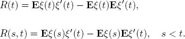
The following descriptive process Q(t) is used to measure the performance of our queueing networks. For each node i = 1, 2, ..., r, let Qi (t) define the number of calls that are being served at the ith node at the instant t. The r-dimensional process Q (t) = (Q1(t),..., Qr(t))′, t ≥ 0, is called the service process of calls for the queueing network.
For most results in the chapter, it is supposed that at the initial instant a network is empty, and there are no calls being served in the network nodes. This means that the network operates in a transient regime. Actually, it is not a crucial assumption, i.e. formulated results are valid not only for an absolutely empty network, but also for the network that is “moderately” loaded from the start. This implies that the number of calls at the initial instant is equal to the certain constant value that does not depend on a series number and, therefore, cannot affect the limit service process. A totally different case is when the starting load of the network is asymptotically increasing in series scheme. In such a situation, the loading process can yield to substantial changes in the representation of the limit process. For this case, we provide conditions under which a multidimensional Ornstein–Uhlenbeck process can be obtained as the limit of the service process.
We now consider a sequence of open multichannel queueing networks indexed by n (series number), where n tends to infinity. Each of these networks is to have the same basic structure as described above. The number of networks nodes remains fixed for all n. On the other hand, the basic stochastic input process ν(t), service times distribution and network initial load are allowed to change with n for different cases. This dependence is indicated by upper index ∙n near the correspondent letter defining input flow or service time distribution.
So, in this section, a class of multichannel networks under consideration is defined. Often for a set of these models, convergence of the service process to a diffusion process can be proved using the local approach, like it is done in the following section.
7.3. Local approach to prove limit theorems
Recall that the diffusion process ξ′(t) = (ξ1(t), ...,ξr(t)) ∈ Rr is defined as a Markov process exhibiting the following local properties for all ε > 0 :
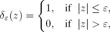
where a(s, t) is a drift vector, b(s, t) is a diffusion matrix, s, t ∈ [0, ∞) ,s < t, x, z ∈ Rr, Δξ = ξ(t) – ξ(s).
Taking into account the local properties, it would be reasonable to seek convergence conditions for a sequence of stochastic processes
to a diffusion process ξ(t) in terms of increments ofξn(t).
In this point, we formulate Gihman’s variant of sufficient conditions of convergence to a diffusion (Gikhman 1969).
Let ξn(t),t ∈ [0,T], n ≥ 1, be a sequence of stochastic processes and let ξ(t), t ∈ [0,T], be a diffusion with the drift vector a(s, t) and the diffusion matrix b(s, t). In order that ξn(t),n ≥ 1, converges to ξ(t) in distribution, it is sufficient that ξn(0) converges to a certain random vector ξo in distribution, and there exists a sequence of partitions of the interval [0,T] by points
and a sequence of families of monotonically increasing σ–algebras ![]() such that the following conditions hold:
such that the following conditions hold:
- – process ξn(t) is
 measurable for t ∈ [0,T], and n = 1, 2, ...;
 - – for any ε>0,z Rr and n
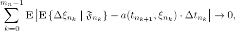
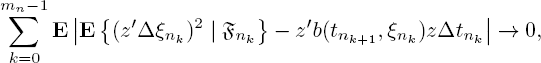

Conditions [7.4]–[7.6] correspond to the local properties [7.1]–[7.3] and mean proximity of the local characteristics (in terms of increments) of the prelimit and limit processes.
Note that in order to provide such approximation, in addition to conditions [7.4]–[7.6], it is necessary for a(s, x) and b(s, x) to be “fairly smooth” functions. The rigorous statement of these conditions can be found in Gikhman (1969). In the current section, all coefficients a(s, x) and b(s, x) of all diffusion processes approximating service processes of queueing networks satisfy the smooth conditions. Therefore, later we always imply that smooth conditions are fulfilled without emphasizing on it.
With that said, checking conditions [7.4] and [7.5] for the service processes of queueing systems and networks reduces to computation and analysis of the first and second conditional moments of increments of the prelimit process. Proof of [7.6] is usually equivalent to testing the Lindeberg condition for some sequence of random variables constructed on the service process.
7.3.1. Network of the [GI|M|∞]r-type in heavy traffic
The local approach is a suitable tool to prove limit theorems provided that the input flow of the network can be defined in a constructive way. Let us consider a multichannel network of the [GI|M|∞]r-type.
To obtain a heavy traffic limit theorem for our sequence of service processes, we need to impose some additional conditions of overloading on the network parameters as n →∞. So, service rates μi, i = 1, 2, ..., r, are assumed to be dependent on the series number n so that the following condition holds.
CONDITION 7. 1. – ![]() = μi, i = 1, 2, ..., r.
= μi, i = 1, 2, ..., r.
In this section, we assume that other parameters of the [GI|M|∞]r-network do not depend on n.
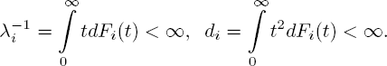
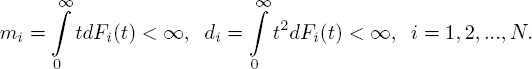
For recurrent input flows ν(i)(t),i = 1, 2, ..., r, we require boundedness of the first and the second moments of interarrival times:
CONDITION 7 . 2 . – For all i = 1, 2 ,..., r
Here, we suppose the network to be empty at the initial instant:
CONDITION 7.3.- Qi(0) = 0 for all i = 1, 2,...,r.
Under conditions 7.1–7.3 for the open [GI∣M∣∞]r-network, we consider the sequence of stochastic processes
where
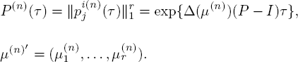
θ′ = (θ1, ..., θr) = λ′(I − P)−1 is a solution of the balance equation for the [GI|M|∞]r-network, P(t) = exp {Δ(μ)(P − I)t} , Δ(x) = ![]() is a diagonal matrix for any vector x′ = (x1 ,..., xr), μ′ = (μ1 ,..., μr), I =
is a diagonal matrix for any vector x′ = (x1 ,..., xr), μ′ = (μ1 ,..., μr), I = ![]() is the identity matrix.
is the identity matrix.
For ξn(t), the following result holds true.
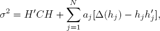
THEOREM 7.1.– Let for a queueing network of the [GI∣M∣∞]r-type conditions 7.1–7.3 be satisfied, Fi(t), i = 1, 2 ,..., r, be a non-lattice function and the spectral radius of the switching matrix P be strictly less than one. Then on any finite interval [0, T], the sequence of stochastic processes ξn(t),n ≥ 1, converges weakly in the uniform topology to a diffusion process ξ(t) (ξ(0) = 0) with drift vector A(x) = A’x and diffusion matrix
where A = Δ(μ)(P − I), σ2 = ![]() i = 1, 2, ...,r.
i = 1, 2, ...,r.
SKETCH OF THE PROOF.- Let us check conditions [7.4]-[7.6] successively.
As a sequence of monotonically increasing σ-algebras ![]() , we can take the σ-algebras generated by the random variables
, we can take the σ-algebras generated by the random variables
where ![]() is the arrival moment of the kth call in the ith node.
is the arrival moment of the kth call in the ith node.
As a sequence ![]() = 1, 2, ..., we take the sequence of the uniform partitions
= 1, 2, ..., we take the sequence of the uniform partitions
for some α ∈ (0;1/2).
Now, for our case, condition [7.4] takes the form:
The path of the call arrived at the [GI|M|∞]r-network through the kth node can be described by a Markov chain y(k) (t) = {1, 2 ,..., r.r + 1} ,t ≥ 0, y(k) (0) = k, which is defined by the infinitesimal matrix ![]() with the following entries:
with the following entries:
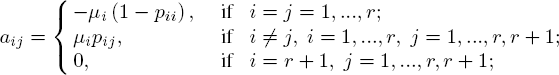
The state r+ 1 for the chain y(k) (t) is an absorbing one. Absorption in the state r+1 means that the call leaves the network. We denote by ![]() the transient probabilities of the chain,
the transient probabilities of the chain,![]() = exp (At).
= exp (At).
Let us connect an r-dimensional process of indicator type
with the chain y(k)(t) as follows:

where e0 is an r-dimensional zero vector, ej is an r-dimensional vector with its jth entry equal to one while the rest of the entries are zero.
If, at the initial instant, a call arrives to the network for its service through the ith node, then the process χ(i)(t) points out the node where the call is staying at the instant t. If χ(i)(t)=e0, it means that the call has already been served before the instant t, and it leaves the network through the (r + 1)th node.
Denote by ![]() i = 1, ...,r, j = 1, 2,..., independent stochastic processes with the same finite-dimensional distributions as ones of χ(i)(t). Then we have the following:
i = 1, ...,r, j = 1, 2,..., independent stochastic processes with the same finite-dimensional distributions as ones of χ(i)(t). Then we have the following:
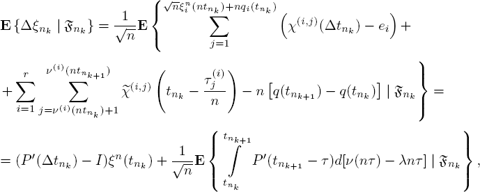
Substituting ![]() in the form [7.8] into [7.4], we obtain:
in the form [7.8] into [7.4], we obtain:

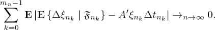
Estimation [7.9] proves validity of [7.4]. Substantially, (P′(Δtnk) − I) ξnk − A′ξnk Δtnk has order (Δtnk)2, therefore

By virtue of the above hypothesis on the sequence of partitions, the second term on the right side of [7.9] has order n−(1/2−α) and converges to zero as well. Similarly, one can check condition [7.5] relating to the diffusion matrix of the limit process.
Condition [7.6] is equivalent to Lindeberg’s condition in the central limit theorem. Thus, the proof of [7.6] can be obtained as a consequence of the following auxiliary result.
LEMMA 7.1.–(See (Anisimov and Lebedev 1992, p. 149) Let ![]() be a sequence of i.i.d. random variables with their distribution dependent on the parameter n (series number), and let
be a sequence of i.i.d. random variables with their distribution dependent on the parameter n (series number), and let ![]() , Var
, Var![]() . Then for any A>0 and any sequence mn → ∞ under n →∞, we have:
. Then for any A>0 and any sequence mn → ∞ under n →∞, we have:

An effective tool to prove the convergence of functionals given for the service process of a network is Billingsley’s test.
LEMMA 7.2.– (See (Billingsley 1999, p.142) Let the sample functions of ξ (t) and ξn(t), n ≥ 1, t ∈ [0,T], belong to the Skorokhod space D[0,T] with probability 1 and the finite-dimensional distributions of ξn (t), n ≥ 1, t ∈ [0,T], are assumed to converge to the finite-dimensional distributions of ξ (t), t ∈ [0,T]. If for any ε > 0
where F(·) is a non-decreasing continuous function on [0, T], then the sequence of stochastic processes ξn (t), n ≥ 1, converges to ξ (t) in the J-topology (Skorokhod’s topology).
In the framework of theorem 7.1, the convergence of ξn (t) to the diffusion ξ (t) can be derived by virtue of[7.10] and Chebyshov’s inequality. Since the limit process ξ (t) has a continuous choice function with probability one, the convergence is in the uniform topology.
This completes the proof of theorem 7.1.
7.4. Limit theorems for networks with controlled input flow
7.4.1. Diffusion approximation of [SM|M|∞]r-networks
Now, let us consider a network of the [SM|M|∞]r-type. In this model, from the outside, a common input flow arrives at the network. The flow is controlled by a semi-Markov process x(t), t ≥ 0, with the state space {1, 2 ,..., N} . It means that the calls’ arrival moments coincide with the jumps time τn, n = 1, 2,..., of x (t). If at τn the process x(t) jumps to the state i, then the arrived call numbered n is directed to the node j with probability hij∙ , ![]() . The matrix
. The matrix ![]() has dimension N × r. By
has dimension N × r. By ![]() , we denote the semi-Markov matrix of the process x(t), and by
, we denote the semi-Markov matrix of the process x(t), and by ![]() , the distribution function of the sojourn time in the state i. The service of calls and the routing algorithm are the same as in the previous model.
, the distribution function of the sojourn time in the state i. The service of calls and the routing algorithm are the same as in the previous model.
Note that input flows ν(i) (t), i = 1, 2, ..., r, into different nodes of the [SM|M|∞]r -network are related.
Instead of condition 7.2 from the previous section, we assume for semi-Markov process x(t) the following:
CONDITION 7.4.– The matrix ![]() of transition probabilities of the embedded Markov chain for x(t) is irreducible, and sojourn times at each node have the first- and second-order moments:
of transition probabilities of the embedded Markov chain for x(t) is irreducible, and sojourn times at each node have the first- and second-order moments:
Under condition 7.4 for F, a stationary distribution (π1, π2 ,..., πN) exists, and Π denotes the matrix of the dimension N × N with N identical lines that are (π1 ,π2 ,..., πN) .
The rate λi,i = 1, 2, ..., r, of the input flow arriving to the ith node, which is used in the centering procedure of the service process, has the form:

In order to formulate a theorem on DA for a [SM|M|∞]r-network, the following limit correlation matrix is needed:
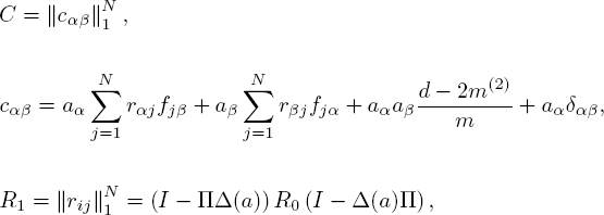
where ![]()
![]() = (hji ,..., hjr) is the jth line of the matrix H, R0 = (I − F + Π)−1 − Π is the potential of the embedded Markov chain.
= (hji ,..., hjr) is the jth line of the matrix H, R0 = (I − F + Π)−1 − Π is the potential of the embedded Markov chain.
We obtain the following result of asymptotic analysis of the stochastic process [7.7] for the [SM|M|∞]r-network in transient and heavy traffic regimes.
THEOREM 7.2.– Let conditions 7.1, 7.3, 7.4 be satisfied for a queueing [SM|M|∞]r- network, and let the spectral radius of the switching matrix P be strictly less than one. Then the sequence of stochastic processes ξn (t), n ≥ 1, converges weakly in the uniform topology on any finite interval [0, T] to a diffusion process ξ (t) (ξ(0) = 0) with drift vector A(x) = A’x and diffusion matrix B(t) = Δ[q′(t)A] − A′Δ[q(t)] − Δ[q(t)]A + σ2, where the matrix σ2 is determined via the network parameters by relations [7.11].
Theorem 7.2 can be proved using the local approach.
Note that models with similar parameters control (the [MSM,Q|MSM,Q|1|∞]r-networks) are investigated under the heavy traffic conditions in Anisimov (2008, pp.164–168), using another technique.
7.4.2. Asymptotics of stationary distribution for [SM|GI|∞]r-networks
In this section, we consider a multichannel [SM|GI|∞]r-network. It means that service times in the jth node are i.i.d. random variables with a distribution function Gj (t ), j = 1, 2, ..., r, t ≥ 0.
At this point, we consider a service process Qi (t) = ![]() t ≥ 0, i = 1, 2, ..., r, where
t ≥ 0, i = 1, 2, ..., r, where ![]() is the number of calls in the jth node at the instant t, provided that the network is empty at the initial instant t = 0, x(0) = i, the arrival moment of the first call is the same as an exit moment τ1 from the state i, and τ1 is distributed in accordance with Fi(t).
is the number of calls in the jth node at the instant t, provided that the network is empty at the initial instant t = 0, x(0) = i, the arrival moment of the first call is the same as an exit moment τ1 from the state i, and τ1 is distributed in accordance with Fi(t).
Denote multivariate generating functions of the vectors Qi (t),i = 1, 2 ,..., N, by Φi(t, z),t ≥ 0, |z| ≤ 1.
Let LT, 0 < T< ∞, be a complete metric space of vector functions
with components Φi(t, z) determined for t ≥ 0, │z│≤ 1, measurable over t which are probability generating functions of z. A distance between Φ, Φ* ∈ LT is equal
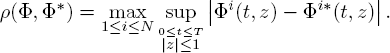
It can be shown that for any T > 0 the generating functions Φi(t, z), 0 ≤ t ≤ T, |z| ≤ 1, are the unique solution of the following system of integral equations:

Under 0 ≤ t ≤ T the solution belongs to LT.
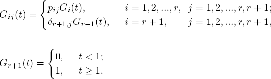
In the right part of[7.12],![]() are the transient probabilities of the semi-Markov process y(t) ∈ (1, 2 ,..., r, r + 1), t ≥ 0, given by the semi-Markov matrix
are the transient probabilities of the semi-Markov process y(t) ∈ (1, 2 ,..., r, r + 1), t ≥ 0, given by the semi-Markov matrix ![]() :
:
Now we reference one result.
THEOREM 7.3.– (See (Lebedev 2002b)) Let the matrix F(t) be non-lattice, the matrix F = F(+∞) be irreducible and π1,π2 ,..., πN be the stationary probabilities of F. If
and the spectral radius of the switching matrix P is strictly less than one, then there exists a stationary regime for the service process Q(t), and

For non-Poisson input flow, the stationary distribution has a complex structure. The stationary probabilities do not have a multiplicative form which is valid for the wide class of Markov stochastic networks. Properties of stationary distribution for some special cases of the [SM|GI|∞]r-models were studied in Lebedev (2002a). It was shown that using binomial moments is an effective tool for investigating the stationary regime of such multichannel networks.
7.4.3. Convergence to Ornstein–Uhlenbeck process
In this section, we consider [SM|M|∞]r-models. In conditions for existence of a stationary regime, we denote by Q = (Q1 ,..., Qr)′ a random vector corresponding to the stationary distribution. Let us proceed with the asymptotic analysis of the vector sequence Q = Qn in heavy traffic for an [SM|M|∞]r-network.
THEOREM 7.4.– Suppose conditions 7.1 and 7.4 hold for an [SM|M|∞]r-network, F(t) is a non-lattice function, and the spectral radius of the switching matrix P is strictly less than one. Then
where the random vector ζ0 has Gaussian distribution with Eζ0 = 0, and the following correlation matrix:
The matrix σ2 is given by [7.11].
A proof of theorem 7.4 is based on the functional limit theorem 7.2.
Assume that a [SM|M|∞]r-network operates in a stationary regime while conditions 7.1 and 7.4 of overloading hold. Then the sequence
satisfies the following result.
THEOREM 7.5.– If a queueing [SM|M|∞]r-network operates in a stationary regime and the assumptions of theorem 7.4 are satisfied, then the sequence of stochastic processes ζn(t),n ≥ 1, converges weakly in the uniform topology on any finite interval [0,T] to an r-dimensional stationary diffusion Ornstein–Uhlenbeck process ![]() with the drift vector A(x) = A’x and the diffusion matrix
with the drift vector A(x) = A’x and the diffusion matrix
PROOF.– The r-dimensional Ornstein–Uhlenbeck process with the drift A(x) and the diffusion matrix B given by theorem 7.5 has stationary Gaussian distribution with zero mean and correlation matrix [7.15]. Therefore, theorem 7.4 provides weak convergence of an initial distribution for the prelimit and limit processes ![]() . Validity of other conditions of local approach can be established similarly to that in theorem 7.1.
. Validity of other conditions of local approach can be established similarly to that in theorem 7.1.
7.5. Gaussian approximation of networks with input flow of general structure
7.5.1. Gaussian approximation of [G|M|∞]r-networks
Now we consider a case without any restrictions imposed on the structure of the input flow ν(t) = (v(1)(t),..., ν(r)(t))′.
Condition 7.1 is supposed to be fulfilled for service rates μi,i = 1, 2, ..., r, and for the input flow we now assume that the following property holds instead of conditions 7.2 and 7.4.
CONDITION 7.5.– There exist constants λi ≥ 0,i = 1, 2,...,r, λ1 + ... + λr = 0, such that
as n →∞, where W(t) is an r-dimensional Brownian motion with zero mean ![]() and the correlation matrix EW(1)W′(1) = σ2 =
and the correlation matrix EW(1)W′(1) = σ2 = ![]() symbol
symbol ![]() denotes weak convergence in the uniform topology, n is a series number.
denotes weak convergence in the uniform topology, n is a series number.
In order to construct a limit process for the sequence of stochastic processes

where θ′ = (θ1 ,..., θr) = λ′ (I − P)−i is a solution of the balance equation for the [G|M|∞]r-network, λ′ = (λ1 ,..., λr), we consider two independent Gaussian processes ξ(1)(t) and ξ(2)(t) with zero means and the following correlation matrices:

The summarized process ξ(1) (t)+ ξ(2) (t) describes asymptotic behavior of the sequence of stochastic processes ξn(t).
THEOREM 7.6.– (See (Lebedev 2003)) Let conditions 7.1, 7.3 and 7.5 be satisfied for a [G|M|∞]r-network, and assume the spectral radius of the switching matrix P to be strictly less than one. Then, the sequence of stochastic processes ξn(t),n ≥ 1, converges weakly in the uniform topology on any finite interval [0, T] to ξ(1)(t)+ ξ(2)(t).
The proof of theorem 7.6 is based on some auxiliary results.
LEMMA 7.3.– The finite-dimensional distributions of ![]() coincide with finite-dimensional distributions of the Gaussian process ξ(1)(t).
coincide with finite-dimensional distributions of the Gaussian process ξ(1)(t).
This result can be proved in virtue of properties of stochastic integrals over a Gaussian process with independent increments.
Service of a call in nodes of our network is independent of other calls. In order to define the service process in a constructive way, we use the process of indicator type ![]() , t ≥ 0, i = 1,..., r, introduced in section 7.3.1.
, t ≥ 0, i = 1,..., r, introduced in section 7.3.1.
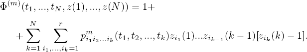
For any natural number N and z′(k) = (z1(k),..., zr(k)), k = 1, 2,...,N, |z(k)| ≤ 1, we denote the joint generating function of the vectors χ(i)(t1) ,..., χ(i)(tN), 0 < t1 < ...< tN, by Φ(i) = Φ(i) (z(1) , ..., z(N), t1 ,..., tN) ,i = 1, 2, ..., r. The following formula takes place for Φ = (Φ(1) ,..., Φ(r))′.
LEMMA 7.4.– For any N = 1, 2,... and 0 < t1 < ... < tN

where ![]() is an r-dimensional vector consisting of ones, Δtk = tk − tk−1 (t0 = 0), k = 1, 2 ,..., N.
is an r-dimensional vector consisting of ones, Δtk = tk − tk−1 (t0 = 0), k = 1, 2 ,..., N.
The proof of lemma 7.4 can be derived by induction over N.
Returning to theorem 7.6, we note that its proof can be obtained from lemmas 7.3 and 7.4, and it is composed of two parts. First, convergence of finite-dimensional distributions is established. Second, convergence in the uniform topology is verified. Arguments of the proof use the method of characteristic functions and representation of the service process under fixed path of input flow as a sum of indicator processes with necessary calculations.
It should be noted that the first term of the limit process is connected with fluctuations of the input flow, and the second one with fluctuations of service time in the network nodes.
Let us prove that the limit Gaussian process in theorem 7.6 is a diffusion. With this aim in view, Markovian property of the limit process has to be proved.
7.5.2. Criterion of Markovian behavior for r-dimensional Gaussian processes
In a one-dimensional case, there is a criterion for Gaussian processes in terms of necessity and sufficiency to verify the Markovian property (see (Feller 1966, theorem 1, p. 94)). The principle condition of the criterion is written in terms of correlations and corresponds to the characteristic property of the exponential function. It is quite convenient to verify it in practice. In the multidimensional case, the situation becomes more complicated and there is no general criterion. We present a variant of the sufficient conditions for the Markovian property of r-dimensional Gaussian processes from Lebedev (2001) and apply this criterion to the limit process in theorem 7.6.
Let![]() be an r-dimensional Gaussian process with zero mean
be an r-dimensional Gaussian process with zero mean
and correlation matrices
THEOREM 7.7.– (See (Lebedev 2001; Livinska and Lebedev 2016)) Let for some matrix A and for all s, t (0 ≤ s < t) the functions R(s) and R(s, t) be related in the following way:
Then the r-dimensional Gaussian process ξ(t) is a Markov process, and the conditional distributions ![]() ,
, ![]() (σ-algebra of Borel subsets of
(σ-algebra of Borel subsets of ![]() ), is Gaussian with mean vector P′(t − s)x and correlation matrix R(t) − P′(t − s)R(s)P(t − s).
), is Gaussian with mean vector P′(t − s)x and correlation matrix R(t) − P′(t − s)R(s)P(t − s).
Note that if GA is the set of Gaussian processes for which the condition of theorem 7.7 is valid and the corresponding matrices are the same (equal A), then GA satisfies the closure condition: a linear combination of two independent processes from GA belongs GA . Thus, we obtain the following interesting fact: the sum of two independent Markov GA-processes is a Markov process. Note also that the multidimensional Ornstein–Uhlenbeck process satisfies the condition of theorem 7.7.
Let us apply the criterion of Markov behavior given by theorem 7.7 to the limit Gaussian process ![]() in theorem 7.6.
in theorem 7.6.
COROLLARY 7.1.– Let conditions of theorem 7.6 be fulfilled. Then the sequence of stochastic processes ξn(t), n ≥ 1, converges weakly in the uniform topology on any finite interval [0, T] to diffusion ξ(t) (ξ(0) = 0) with the drift vector A(x) = A’x and the diffusion matrix
If we denote the corresponding correlation matrices of the process ![]() by R(t), R(s, t), s < t, then the conditions of theorem 7.7 are satisfied for them with A = Δ(μ)(P − I). So,
by R(t), R(s, t), s < t, then the conditions of theorem 7.7 are satisfied for them with A = Δ(μ)(P − I). So, ![]() is a Markov diffusion process. Drift vector and diffusion matrix are determined by the form of conditional distribution
is a Markov diffusion process. Drift vector and diffusion matrix are determined by the form of conditional distribution ![]() ,
, ![]()
7.5.3. Non-Markov Gaussian approximation of  -networks
Now, in contrast to sections 7.5.1 and 7.5.2, the distribution function Gi(t), i = 1, 2, ..., r, of service times in the network nodes has general form and the memorylessness property can be not fulfilled.
The path of a call in such a network can be described by a semi-Markov process y(t), t ≥ 0, with the set of states {1, 2,...,r,r +1} and with its semi-Markov matrix ∣∣![]() defined in section 7.4.2.
defined in section 7.4.2.
In accordance with the construction, the state r +1 is an absorbing one for the process y(t). Recall that transient probabilities of the semi-Markov process y(t) are ![]() = P (y(t) = j | y(0) = i), P(t) =
= P (y(t) = j | y(0) = i), P(t) = ![]() .
.
In order to define the heavy traffic transient regime for the [G|GI|∞]r-network, we keep conditions 7.3 and 7.5 for initial distribution and for input flow, but instead of condition 7.1 we require the following.
CONDITION 7.6.– ![]() , as n → ∞, i = 1, 2,...,r,
, as n → ∞, i = 1, 2,...,r,
where ![]() means weak convergence of distribution functions.
means weak convergence of distribution functions.
The main objective of this section is to study limit behavior of the sequence of stochastic processes

where ![]() are the transient probabilities of the semi-Markov process yn(t) defined likewise y(t),t ≥ 0, with changing
are the transient probabilities of the semi-Markov process yn(t) defined likewise y(t),t ≥ 0, with changing ![]()
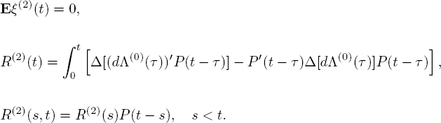
In this regard, let us consider two mutually independent Gaussian processes ξ(1) (t) and ξ(2) (t),t ≥ 0, with zero means and correlation matrices in the following form:
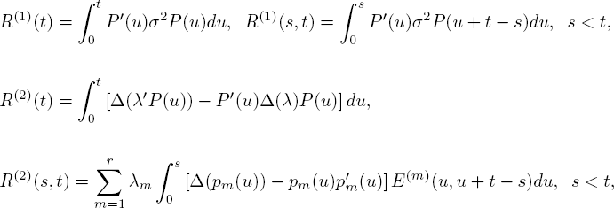
where ![]() is the mth-line of the matrix P(t), and for s < t,
is the mth-line of the matrix P(t), and for s < t, ![]()

If the [G|GI|∞]r-network operates under heavy traffic transient conditions, then the next result holds for the normalized service process ξn(t), n ≥ 1.
THEOREM 7.8.– Let a queueing [G|GI|∞]r-network satisfy conditions 7.3, 7.5 and 7.6, and let the spectral radius of the switching matrix P be strictly less than one. Then the sequence of stochastic processes ξn(t), n ≥ 1, converges in the uniform topology on any finite interval [0, T] to ξ(1)(t) + ξ(2)(t).
Substantially, theorem 7.8 is an analogue to theorem 7.6. The main difference is that the limit process is a non-Markov process if the distribution function of service times is not exponential at least in one network node.
The sketch of the proof is similar as well. The statement of lemma 7.3 for the [G|GI|∞]r-network will be the same if we consider the matrix of transient probabilities of semi-Markov process y(t) as the matrix P(t).
Going forward, we need the following result instead of lemma 7.4.
Let 0 ≤ t1 < t2 < ... < tk, and
where the distribution function of sojourn time of y(t) in the initial state m is assumed to be the same as Gm(t).
Functions ![]() (t1 , t2 , ..., tk) are uniquely determined by the sequence of systems of Markov renewal integral equations
(t1 , t2 , ..., tk) are uniquely determined by the sequence of systems of Markov renewal integral equations

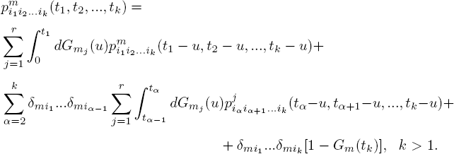
LEMMA 7.5.– If the spectral radius of the matrix P is strictly less than one, then for any N = 1, 2, ... and 0 < t1 <...< tN we have
Like the statement of lemma 7.4, the last result can be obtained by the method of mathematical induction with respect to N.
The above models have one point in common: their parameters do not depend on time. Surely, it constricts the applications field. Especially, this point is sensitive when one simulates input flows with their real-life rates dependent on time. Further, within the framework of the simplest Markov models, we remove this restriction.
7.6. Limit processes for network with time-dependent input flow
7.6.1. Gaussian approximation of  -networks in heavy traffic
Let us consider a network with a non-homogeneous Poisson input flow of calls ν(i) (t) arriving at the ith node, i = 1, 2, ..., r. Suppose Λi(t) is the leading function of ν(i)(t). Service times in the ith node are independent exponentially distributed random variables with rate μi. As before, the r-dimensional service process of calls Q(t) = (Q1(t),..., Qr(t))′, t ≥ 0, is studied.
The heavy traffic regime for the ![]() -network is determined by condition 7.1 and the following condition on input flow parameters.
-network is determined by condition 7.1 and the following condition on input flow parameters.
CONDITION 7.7.– Input flows depend on n in such a way that on any finite interval
where C[0,T] is the set of continuous on [0, T] functions, the symbol ![]() stands for convergence in the uniform topology.
stands for convergence in the uniform topology.
Let us consider two cases that are important for applications when condition 7.7 is valid. We temporarily assume that the Poisson flows ν(i) (t), i = 1, 2 ,..., r, are regular: Λi(t)= ![]() , where λi(u) is the instant value of the parameter.
, where λi(u) is the instant value of the parameter.
7.7a If λi (t) is a periodic function with period Ti, then condition 7.7 holds with ![]()
7.7b If limt→∞ λi(t) = λi > 0, then condition 7.7 holds with ![]()
Note, that networks with a periodic input flow are studied in more details in Livinska and Lebedev (2018).
In the context of conditions 7.1 and 7.7, we consider the sequence of stochastic processes:
![]()
![]() are entries of the matrix
are entries of the matrix
In order to describe the limit of the sequence of stochastic processes ξn (t) as n → ∞, we introduce two independent Gaussian processes
The process ξ(1)(t) is determined by zero mean:
and by the correlation matrices:

where ![]() P(τ) = exp{Δ(μ)(P − I)τ.
P(τ) = exp{Δ(μ)(P − I)τ.
For the process ![]() :
:
The following result gives an approximation for the service process of an ![]() -network under heavy traffic conditions 7.1 and 7.7.
-network under heavy traffic conditions 7.1 and 7.7.
THEOREM 7.9.– Let conditions 7.1 and 7.7 take place for an ![]() -network, and let the network be empty at the initial instant t = 0: Qi(0) = 0,i = 1, 2 ,..., r. Then, the sequence of stochastic processes ξn (t) converges on any finite interval [0, T] as n → ∞ to the process ξ(1)(t) + ξ(2)(t) in the uniform topology.
-network, and let the network be empty at the initial instant t = 0: Qi(0) = 0,i = 1, 2 ,..., r. Then, the sequence of stochastic processes ξn (t) converges on any finite interval [0, T] as n → ∞ to the process ξ(1)(t) + ξ(2)(t) in the uniform topology.
SKETCH OF THE PROOF OF THEOREM 7.9.– The proof follows from some auxiliary results and is similar to the proof of theorem 7.6.
In the case of non-homogeneous Poisson input flow, we have to prove the next property which is parallel to condition 7.5 supposed a priori.
LEMMA 7.6.–Let νn(t) be a non-homogeneous Poisson process with the leading function Λ(n)(t) such that condition 7.7 is valid. Then the sequence of stochastic processes W(n)(t) = ![]() n ≥ 1, converges in the uniform topology on any finite interval [0, T] to a Wiener process W(0)(t) with EW(0)(t) = 0and VarW(0)(t) = Λ(0)(t).
n ≥ 1, converges in the uniform topology on any finite interval [0, T] to a Wiener process W(0)(t) with EW(0)(t) = 0and VarW(0)(t) = Λ(0)(t).
Convergence of finite-dimensional distributions of the process W(n) (t) to W(0) (t) follows from the fact that for any natural number N and instants 0 < t1 < ... < tN the joint characteristic function of the distribution of νn(t1) ,..., νn(tN) is equal to
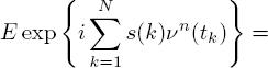
where (s(1) ,..., s(N)) ∈ ![]() ,t0 = 0.
,t0 = 0.
Now, in order to prove the convergence in the uniform topology, it is sufficient to check the following condition for any ε > 0 :
Based on Chebyshov inequality, we have the upper estimate:

On the other hand, condition 7.7 implies that
So, [7.16] follows from [7.17] and [7.18].
Lemma 7.6 is proved.
Throughout the section, ![]() = 1, 2,..., r, denote independent Wiener processes with zero mean and
= 1, 2,..., r, denote independent Wiener processes with zero mean and ![]() If condition 7.7 holds, they approximate the input flows ν(i)n(t).
If condition 7.7 holds, they approximate the input flows ν(i)n(t).
For W(0)′ (t) = ![]() we need the result given by lemma 7.3. Lemma 7.4 have to be satisfied as well. So, like in the case for theorem 7.6, the proof of theorem 7.9 can be obtained from lemmas 7.3, 7.4 and 7.6.
we need the result given by lemma 7.3. Lemma 7.4 have to be satisfied as well. So, like in the case for theorem 7.6, the proof of theorem 7.9 can be obtained from lemmas 7.3, 7.4 and 7.6.
It is easily observed that the limit of ξn(t) is a Markov Gaussian process. However, it can be presented as a diffusion process due to theorem 7.7.
THEOREM 7.10.– Let an ![]() -network be empty at the initial instant t = 0, let conditions 7.1 and 7.7 hold and
-network be empty at the initial instant t = 0, let conditions 7.1 and 7.7 hold and ![]() , i = 1, 2 ,..., r. Then, the sequence of stochastic processes ξn(t) ,n ≥ 1, weakly converges on any finite interval [0, T] in the uniform topology to the r-dimentional diffusion process ξ(0)(t) with the drift vector A(x) = A’x and the diffusion matrix
, i = 1, 2 ,..., r. Then, the sequence of stochastic processes ξn(t) ,n ≥ 1, weakly converges on any finite interval [0, T] in the uniform topology to the r-dimentional diffusion process ξ(0)(t) with the drift vector A(x) = A’x and the diffusion matrix
where ![]() ,
,
The form of the limit process as a multidimensional diffusion is attractive because a diffusion process is determined only by its local characteristics and one can use the developed tools of Markov diffusion processes for the analysis of its functionals. However, now the limit process does not reflect in detail the structure of the prelimit service process.
7.6.2. Limit process in case of asymptotically large initial load
Let us consider a case when the number of calls being served in the ![]() - network at the initial instant of time depends on n and increases as n → ∞. In this case, the service process of calls that were initially located at the network can converge to a non-zero limit, and this term can enter into the overall limit process. So, fulfillment of the following condition is required here instead of
- network at the initial instant of time depends on n and increases as n → ∞. In this case, the service process of calls that were initially located at the network can converge to a non-zero limit, and this term can enter into the overall limit process. So, fulfillment of the following condition is required here instead of ![]() = 0, i = 1, 2, ..., r :
= 0, i = 1, 2, ..., r :
CONDITION 7.8.– ![]() =
= ![]() , i = 1, 2 ,..., r, where
, i = 1, 2 ,..., r, where ![]()
![]() is a fixed vector in
is a fixed vector in
![]() , [∙] is the integer part of a number.
, [∙] is the integer part of a number.
Here, we will consider an open ![]() -network with periodic input flow. As before, let θ′ = (θ1 ,..., θr) = λ′(I − P)−1 be a solution of the balance equation, where λ′ = (λ1 ,..., λr), and in this case
-network with periodic input flow. As before, let θ′ = (θ1 ,..., θr) = λ′(I − P)−1 be a solution of the balance equation, where λ′ = (λ1 ,..., λr), and in this case ![]() , i = 1, 2,..., r.
, i = 1, 2,..., r.
Next, we study the asymptotic behavior of the sequence of stochastic processes
With this in mind, we introduce in addition a Gaussian process ξ(3)(t) that does not depend on the previously introduced processes ξ(1)(t) and ξ(2)(t). This process ξ(3)(t) is determined by the mean values
and by the correlation matrices

THEOREM 7.11.– (See (Lebedev and Livinska 2018)) Suppose that an ![]() – network with a periodical input flow has the spectral radius of its switching matrix strictly less than 1, and let conditions 7.1, 7.7a and 7.8 be satisfied. Then, the sequence of stochastic processes ηn(t) converges as n → ∞ to ξ(1) (t) + ξ(2) (t) + ξ(3) (t) in the uniform topology on any finite interval [0, T].
– network with a periodical input flow has the spectral radius of its switching matrix strictly less than 1, and let conditions 7.1, 7.7a and 7.8 be satisfied. Then, the sequence of stochastic processes ηn(t) converges as n → ∞ to ξ(1) (t) + ξ(2) (t) + ξ(3) (t) in the uniform topology on any finite interval [0, T].
In comparison with the statement of theorem 7.9, the additional summand ξ(3)(t) of the limit process is associated with fluctuations of service times of calls located in network nodes at the initial instant t = 0.
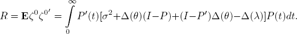
It is not difficult to check that for correlation matrices, we have:
So, theorem 7.11 implies the following result for ηn(t).
COROLLARY 7.2.– Let for an open ![]() -network conditions 7.1, 7.7a and 7.8 be satisfied. Then the sequence of stochastic processes ηn(t) converges as n → ∞ in the uniform topology on any finite interval [0, T] to an r-dimensional Ornstein-Uhlenbeck diffusion process η(0) (t) in transient regime (η(0)(0) = η(0)) with the following correlation characteristics:
-network conditions 7.1, 7.7a and 7.8 be satisfied. Then the sequence of stochastic processes ηn(t) converges as n → ∞ in the uniform topology on any finite interval [0, T] to an r-dimensional Ornstein-Uhlenbeck diffusion process η(0) (t) in transient regime (η(0)(0) = η(0)) with the following correlation characteristics:

7.7. Conclusion
In this chapter, we investigate the asymptotic behavior of the service process of calls for some stochastic networks with infinite number of servers in each node under heavy traffic assumptions. It is convenient to use the local approach for proving DA for this class of network, or to use constructive probabilistic methods for the Gaussian approximation of service process of the network.
We consider networks with input flows of different structure and with exponential and general service. Networks with time-dependent Poisson input flow are considered in two different cases of starting load: first, the number of calls in the initial instant is assumed to be equal to zero; second, this number is assumed to increase with a series number increasing. For models with exponential service, DA is proved either by the local approach or by proving a functional limit theorem on convergence to Gaussian process and checking Markovian property of the limit process using correspondent criterium presented in the chapter. Note that if a distribution function of the service time is not exponential at least in one node, then an accumulation of aftereffect takes place during servicing, and the limit process is not a Markov process. More networks with such service are studied, for example, in Lebedev (2002a, 2002b) and in Livinska (2016).
As for Gaussian approximation provided in the chapter, it is proved that under formulated heavy traffic conditions, the normalized service process has Gaussian process as a limit in the uniform topology. So, jump-wise service processes are approximated by Gaussian processes with continuous paths and simpler structure. It is significant that the limit process is decomposed into the sum of independent Gaussian processes. In the case of the fixed initial load, it has two summands ξ(1) (t) and ξ(2) (t). The part ξ(1) (t) of the limit process is associated with fluctuations of an input flow, and ξ(2) (t) is associated with fluctuations of service times. In the case of asymptotically large initial load, the third term ξ(3) (t) appears in the sum. It is connected with fluctuations of service times of calls located in the network nodes at the initial instant. Moreover, in the case of asymptotically large load, the limit process is a multidimensional Ornstein–Uhlenbeck diffusion process. For all cases, the approximating Gaussian processes are constructed with their characteristics written in explicit form via the network parameters.
Note also that convergence to Gaussian process is proved in the uniform topology. This type of convergence of stochastic processes gives us a possibility to calculate functionals related with the processes and to solve optimization problems (see, for example, Lebedev and Makushenko (2012)).
Some studies of similar multichannel stochastic networks with time-dependent input flow and different types of service can be found in Lebedev (2017), Lebedev and Livinska (2018), Livinska (2016), Livinska and Lebedev (2018). Networks with input flow controlled by a Markov process were investigated in Lebedev and Livinska (2017).
7.8. Acknowledgements
We would like to thank the editors and the anonymous referees for their valuable suggestions.
7.9. References
Anisimov, V.V. (1995). Switching processes: Averaging principle, diffusion approximation and applications. Acta Applicandae Mathematicae, Kluwer, The Netherlands, 40(2), 95–141.
Anisimov, V.V. (2002). Diffusion approximation in overloaded switching queueing models. Queueing Syst., 40(2), 141–180.
Anisimov, V.V. (2008). Switching Processes in Queueing Models. ISTE Ltd, London, and Wiley, New York.
Anisimov, V.V. (2010). Switching queueing networks. In Performance Evaluation and Applications, D. Kouvatsos (ed.), Springer-Verlag. 5233, 258–283.
Anisimov, V.V. and Lebedev, E.A. (1992). Stochastic Queueing Networks. Markov Models. Lybid, Kiev.
Basharin, G., Bocharov, P. and Kogan, J. (1989). Analysis of Queues in Computing Networks. Nauka, Moscow (in Russian).
Bernstein, S.N. (1934). Principes de la théorie des équations différentielles stochastiques. Proceedings of the Phy. Math. Inst. Named Steklov, 5, 95–124.
Billingsley, P. (1999). Convergence of Probability Measures. John Wiley & Sons, Inc., NewYork.
Borovkov, A.A. (1980). Asymptotic Methods in Queueing Theory. Nauka, Moscow (in Russian).
Decreusefond, L. and Moyal, P. (2008). A functional central limit theorem for the M/GI/∞ queue. Ann. Appl. Probab., 186, 156–178.
Dvurečenskij, A., Kulyukina, L.A. and Ososkov, G.A. (1981). Estimations of track ionization chambers. Transactions of United Nuclear Research Institute, Dubna.
Feller, W. (1966). An Introduction to Probability Theory and Its Applications, vol. 2. John Wiley and Sons, Inc., New York.
Fralix, B.H. and Adan, I.J.B.F. (2009). An infinite-server queue influenced by a semi-Markovian environment. Queueing Syst., 61, 65–84.
Gikhman, I.I. (1969). On convergence to Markov processes. Ukr. Math. J., 21(3), 312–320.
Gikhman, I.I. and Skorokhod, A.V. (1982). Stochastic Differential Equations. Naukova Dumka, Kiev (in Russian).
Gnedenko, B.V. and Kovalenko, I.N. (2013). Introduction to Queueing Theory. URSS, Moscow (in Russian).
Khinchin, A.Y. (1936). Asymptotic Principles of Probability Theory. ONTI NKTP USSR, Moscow (in Russian).
Korolyuk, V.S. and Korolyuk, V.V. (1999). Stochastic Models of Systems. Kluwer, Dordrecht.
Korolyuk, V.S. and Limnios N. (2004). Average and diffusion approximation for evolutionary systems in an asymptotic split phase state. Ann. Appl. Prob., 14(1), 489–516.
Korolyuk, V.S. and Limnios, N. (2005). Stochastic Systems in Merging Phase Space. World Scientific, Singapore.
Korolyuk, V.S., Korolyuk, V.V. and Limnios N. (2009). Queuing systems with semi-Markov flow in average and diffusion approximation schemes. Metodol. Comput. Appl. Probab., 11, 201–209.
Lebedev, E.A. (2001). On the Markov property of multivariate Gaussian processes. Bulletin of Kiev Univ. Series: Phys.-Math., 4, 287–291.
Lebedev, E.A. (2002a). Networks of infinite server queues. ESM’2001 Conference Proceedings, Darmstadt, Germany.
Lebedev, E.A. (2002b) Stationary regime and binomial moments for networks of the type [SM|GI|∞]r. Ukr. Math. J., 54(10), 1371–1380.
Lebedev, E.A. (2003). A limit theorem for stochastic networks and its applications. Theor. Probab. and Math. Statist., 68, 81–92.
Lebedev, E.A. and Livinska, H. (2017). On stationary regime for queueing networks with controlled input. WSEAS Trans. on Systems and Control, 12, 9–13.
Lebedev, E.A. and Livinska, H. (2018). On Gaussian approximation of queueing networks with different starting load. Commun. Comp. Inf. Sci., 912, 27–38.
Lebedev, E.A. and Livinska, H. (2019). Multi-channel queueing networks with input flow controlled by semi-Markov process, Math. Comput. Sci. [Online]. Available: https://doi.org/10.1007/s11786-019-00398–4.
Lebedev, E.A. and Makushenko, I.A. (2012). Optimal Partitioning of External Load in Multi-channel Queuing Networks. V.I. Vernadsykiy Library, Kyiv.
Lebedev, E.A., Chechelnitsky, A.A. and Livinska, H.V. (2017). Multi-channel networks with interdependent input flows in heavy traffic. Theor. Probab. and Math. Statist., 97, 109–119.
Livinska H. (2016). A limit theorem for non-Markovian multi-channel networks under heavy traffic conditions. Theor. Probab. and Math. Statist., 93, 113–122.
Livinska, H. and Lebedev E.O. (2015). Conditions of Gaussian non-Markov approximation for multi-channel networks. Proceedings of the 29-th Euro. Conf. on Modelling and Simul. ECMS-2015. Albena, Bulgaria, 642–649.
Livinska, H. and Lebedev, E. (2016). Gaussian and diffusion limits for multi-channel stochastic networks. J. Math. Sci., 218(3), 328–334.
Livinska, H. and Lebedev, E. (2018). On transient and stationary regimes for multi-channel networks with periodic inputs. Appl. Math. and Comput., 319, 13–23.
Mandelbaum, A. and Pats, G. (1995). State-dependent queues: Approximations and applications. In Proc. of the IMA. Stochastic networks, F.P. Kelly and R.J. Williams, (eds), Springer, New York, 239–282.
Mandelbaum, A. and Pats, G. (1998). State-dependent stochastic networks. Part I: Approximations and applications with continuous diffusion limits. Ann. Appl. Prob., 8(2), 569–646.
Mandelbaum A., Masey W. and Reiman M. (1998). Strong approximation for Markovian service networks. Queueing Syst., 30(1,2), 149–202.
Massey, W.A. and Whitt, W. (1993). Networks of infinite-server queues with nonstationary Poisson input. Queueing Syst., 13, 183–250.
Massey, W.A. and Whitt, W. (1994). A stochastic model to capture space and time dynamics in wireless communication systems. Prob. Eng. Inf. Sci., 8, 541–569.
Matis, J.H. and Wehrly, T.E. (1990). Generalized stochastic compartmental models with Erlang transit times. J. Pharmac. Bioph., 18, 589–607.
Moiseev, A. and Nazarov, A. (2015). Infinite-server Queueing Systems and Networks. NTL Publishing, Tomsk (in Russian).
Moiseev, A. and Nazarov, A. (2016). Queueing network M AP − ![]() with high-rate arrivals. Eur. J. Oper. Res., 254(1), 161–168.
with high-rate arrivals. Eur. J. Oper. Res., 254(1), 161–168.
Nazarov, A. and Moiseev, A. (2014). Investigation of the queueing network GI – ![]() by means of the first jump equation and asymptotic analysis. In DCCN 2013, CCIS 279, V. Vishnevsky et al. (ed.). Springer, 229–240.
by means of the first jump equation and asymptotic analysis. In DCCN 2013, CCIS 279, V. Vishnevsky et al. (ed.). Springer, 229–240.
Nazarov, A. and Tuenbaeva, A.N. (2009). Investigation of mathematical model of communication network with unsteady flow of requests. Transp. and Telecom., 4, 28–34.
Prokhorov, Y.V. (1956). Convergence of stochastic processes and limit theorems of probability theory. Theor. Probab. and Appl., 1(2), 177–238.
Puhalskii, A.A. and Reed, J.E. (2008). On many-server queues in heavy traffic. Ann. Appl. Probab., 20, 129–195.
Reiman, M. (1984). Open queueing networks in heavy traffic. Math. Oper. Res., 9(3), 441–458.
Skorokhod, A.V. (1956). Limit theorems for stochastic processes. Theor. Probab. and Math. Statist., 1(3), 289–319.
Whitt, W. (1982). On the heavy-traffic limit theorem for GI/G/∞ queues. Adv. Appl. Probab., 14, 171–190.
Whitt, W. (2016). Heavy-traffic fluid limits for periodic infinite-server queues. Queueing Syst., 84, 111–143.
Whitt, W. (2018). Time-varying queues. Queueing Mod. Serv. Managm., 1(2), 79–164.
Williams, R.J. (1996). On the approximation of queueing networks in heavy traffic. In Stochastic Networks: Theory and Applications, Proceedings of Royal Society Workshop, Edinburgh, 1995, Kelly, F.P., Zachary, S., Ziedins, I. (eds). Oxford University Press, Oxford, 35–56.
Williams, R.J. (2016). Stochastic processing networks. Ann. Rev. Stat. Appl., 3, 323–346.