
3
Diffusion Approximation of Queueing Systems and Networks
Dimitri KOROLIOUK1 and Vladimir S. KOROLIUK2
1Institute of Telecommunications and Global Information Space, National Academy of Sciences of Ukraine, Kiev, Ukraine
2Institute of Mathematics, National Academy of Sciences of Ukraine, Kiev, Ukraine
Markov processes with locally independent increments in Euclidean phase space RN are considered as mathematical models of Markov queueing systems and networks. Average and diffusion approximation schemes with a small series parameter ε > 0 are developed and applied for some concrete queueing systems and networks.
3.1. Introduction
The main problem in the analysis of stochastic queueing systems and networks is to select a class of Markov processes which is adequate for the corresponding queueing processes.
An auxiliary problem is to introduce a series parameter in such a way as to ensure adequate normalization of service processes.
The analytical problem is to choose an adequate method for asymptotic analysis of queueing processes in the diffusion approximation scheme.
For this purpose, the Markov processes with locally independent increments with normalizing series parameter ε → 0(ε >0 ) are considered as adequate processes.
In asymptotical analysis of diffusion approximation schemes, the generator characterization for Markov queueing process is used, as well as the relative limit theorems in series schemes (Korolyuk and Limnios 2005; Korolyuk and Korolyuk 1999).
Limit theorems for switching processes (average and diffusion approximation), applied to the models of queueing systems and networks (branching processes as well), were studied in work by V.V. Anisimov (1995, 2002). A special subclass of switching – recurrent processes of semi-Markov type – was studied and described in a monograph by Anisimov (2008, see also the references therein).
3.2. Markov queueing processes
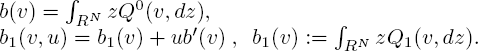
Markov processes ζ(t) , t ≥ 0, with locally independent increments (Korolyuk and Korolyuk 1999) in Euclidean phase space RN can be determined by a generator L on Banach space BRN of real-valued bounded measurable functions φ(u), u ∈ RN, with sup-norm ∣∣φ(u)∣∣ := SUPu∈RN ∣φ(u)∣, as follows:
The kernel Q(u, dz) defining intensities of values of jumps is supposed to be a positive bounded measure:
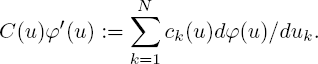
The vector function C(u) = (ck(u), 1 ≤ k ≤ N) sets the velocity of the deterministic drift ρ(t), defined by a solution of the evolutional equation
The second term in [3.1] means the scalar product of two vector functions:
The diffusion component of Markov process is defined by generator

The covariance matrix of diffusion is
The deterministic drift ρ(t) can be considered as a part of a diffusion process with generator
The increments of Markov process ζ(t) on a small time interval Δt can be represented as follows:
where ν(t) is a Markov jump process with generator
The diffusion process w(t) is defined by generator [3.3].
The homogeneous (in time) Markov jump process ν(t), definedby generator [3.3], is considered as a starting point for mathematical modeling of a queueing system.
3.3. Average and diffusion approximation
3.3.1. Average scheme
A queueing process in the average normalized scheme is considered in the following normalization:
That is, the generator of Markov process νε(t) has the following representation:
The main condition in the average approximation scheme is imposed on the asymptotical behavior of the first moment of jumps.
THEOREM 3.1.– (Averaging). Let the following approximation condition hold:
with a negligible residual term
and suppose the existence of a positive solution of equation
Then the normalized queueing process [3.6] converges in distribution, as ε → 0, to a solution ρ(t) of equation [3.10] with initial value ρ0 = P limε→0 ενε(0)
COROLLARY 3.1.- Let the initial value ρ0 ≥ 0 be an equilibrium point for the velocity C(u):
Then the queueing process in the average normalized scheme has an equilibrium point as well:
uniformly on every finite time interval t ∈ [0,T].
PROOF.- (Proof of theorem 3.1). Under the approximation condition [3.8], the generator [3.7], acting on the continuously differentiable function φ(u), has the following asymptotic representation:
where the generator
determines the evolutional equation [3.10]. The residual termθε(u) in [3.12] (different from the term in [3.8]) satisfies the negligible condition [3.9]. Now using martingale characterization of Markov process
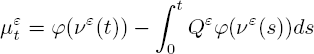
and asymptotical representation [3.12], we get the following asymptotical form for martingale [3.14]:

where the residual term ψtε satisfies the condition
It is easy to verify that the square characteristic of martingale [3.14] admits the representation
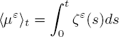
with a random function ζε(s), s ≥ 0, satisfying the condition
Hence, in the previous study (Korolyuk and Korolyuk 1999, theorem 3.4), the weak convergence [3.11] takes place. The limit process ρ(t) is defined by a solution of equation
which is equivalent to evolutional equation [3.10] for the limit process ρ(t).
3.3.2. Diffusion approximation scheme
A Markov queueing process in a diffusion approximation scheme is considered in the following centered and normalized form:
where the Markov jump process νε(t) is determined by generator
The centered function ρ(t) is defined by a solution of evolutional equation
The more general centering scheme with the velocity Cε(u) that depends on a series parameter ε is motivated by a real queueing system with bounded input. In spite of the fact that the Markov jump process νε(t) is homogeneous in time, the normalized centered process [3.19] is heterogeneous, but in a special way, due to the deterministic centered function ρ(t). Meanwhile, the two components, homogeneous in time Markov process ζε(t), ρ(t), t ≥ 0, can be used in the diffusion approximation scheme.
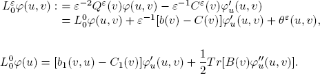
LEMMA 3.1.- The generator of the coupled Markov process ζε(t), ρ(t), t ≥ 0, has the following representation:
where
and the generator Qε(v) acts in the following way:
PROOF OF LEMMA 3.1.-The increments of the first component in [3.19] have the following representation:
According toequation[3.21], one has
Hence
Now the conditional expectation
can be estimated as follows:
Note that, under the condition ζε(t) = u, ρ(t) = v, according to the definition of normalized centered process [3.19], we have:
Therefore, the first term in [3.25] can be estimated as follows:
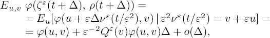
with generator Qε(v) defined in [3.24]. The relations [3.25] and [3.26] imply [3.22]−[3.24]. Note that the intensity kernel Qε(u, dz) defines the intensity of jump values for the process νε(t) under the condition
for a fixed parameter u. The diffusion approximation for a normalized centered queueing process [3.19] is realized under asymptotical representation for infinitesimal characteristics, defined by generator [3.22]-[3.24].
THEOREM 3.2.– (Diffusion Approximation). Let the intensity of jump values of Markov queueing process νε(t) admit asymptotical representation of the first and second moments, as ε → 0:

where the residual terms θε(v, u) in both formulas satisfy the negligibility condition
Let the velocity of the centered function Cε(v) admit asymptotical representation
with a negligible term θε( v):
Then, under the additional balance condition
the normalized centered queueing process ζε(t), defined in [3.19], converges, in distribution, to a diffusion:
The generator of the limit process ζ0(t) is then defined as:
where the centered function ρ(t) is defined by a solution of evolutional equation
with initial value
The initial value of the limit diffusion is defined by the condition
COROLLARY 3.2.-Let the intensity kernel have the following asymptotical representation:
and the kernel Q0(v, dz) be differentiable by v. Then the asymptotical representation [3.27] has the following form:
COROLLARY 3.3.- Let the velocity C (v) of the centered function have an equilibrium point ρ0 ≥ 0: C (ρ0) = 0. Then under the initial conditions [3.34] and [3.35], the limit diffusion of the Ornstein-Uhlenbeck type process is defined by generator
where the drift function is linear with respect to u:
and the covariance matrix is constant:
PROOF.- (Proof of theorem 3.2). The asymptotic representation of generators [3.22]−[3.24] is considered on the set D of real-valued, twice continuously differentiable functions φ(u,v) with compact support.
Taking into account asymptotical representations [3.27] and [3.28] of the first two moments of the jump component and [3.30] for the velocity of centered function, we obtain
As before, the residual term θε(u, v) satisfies the negligiblility condition [3.29]. The balance condition [3.31] yields the following asymptotical representation for generator [3.22]:
Now the martingale characterization of the coupled Markov process ζε(t), ρ(t), t ≥ 0, is the following:

which can be transformed into

with a residual negligible term ![]() satisfying the condition
satisfying the condition
One has to place the following representation of the square characteristic of martingale [3.41]:
with a random function ζε(s), s ≥ 0, which satisfies the compactness condition: for every fixed T , there exists δ > 0 such that
Hence, by the Pattern theorem (Korolyuk and Korolyuk 1999, Theorem 3.4), the following weak convergence (in distribution) takes place:
The limit two-component Markov process ζ0(t), ρ(t), t ≥ 0, is determined by the generator
To complete the proof of theorem 3.2, note that the coupled Markov process ζ0(t), ρ(t), t ≥ 0, with the first component determined by generator [3.32], is defined by generators [3.37] and [3.45]. □
NOTE 3.1.-Using the centered drift function ρε(t), that depends on the series parameter ε, the drift term in [3.32], which is not dependent on u, can be removed. But it is not possible to remove the drift part of the limit diffusion completely.
NOTE 3.2.- The considered class of Markov processes contains “density-dependent population processes” for which the diffusion approximation without a drift component was investigated in the book by Ethier and Kurtz (1986). The limit diffusion is not ergodic despite the fact that the initial process is ergodic.
3.3.3. Stationary distribution
The diffusion approximation of stationary Markov jump processes provides the approximation of their stationary distributions. It means that the stationary distribution density πε(du), ε > 0 , of a normalized and centered queueing process weakly converges, as ε → 0, to stationary distribution density π0(du) of the limit diffusion process.
Essential aspects of this problem are considered in the book by Ethier and Kurtz (1986, Section 4.9). The main idea is to verify the relative compactness of stationary densities πε(du), ε > 0. The most useful approach involves Lyapunov functions V (u), which satisfy the following conditions:
- – V (u) > 0 in some vicinity of zero point u = 0;
- – V(0) = 0;
- – V(u) → ∞ as ∥u∥ → ∞.
In addition, V (u) is an excessive function for generator ![]() of the limit diffusion process:
of the limit diffusion process:
For a given diffusion process, the Itô formula provides a more direct approach (Ethier and Kurtz 1986, Section 4.9, Problem 35).
A weak convergence of stationary distributions is considered for the normalized queueing process with equilibrium point ρ ≥ 0:
The generator of Markov process ζε(t) has the following form:
where
The limit diffusion process in this case, under the conditions of theorem 3.2, is determined by the generator
where
THEOREM 3.3.– (Convergence of stationary distributions). Consider a Lyapunov function V (u) for generator [3.49], which satisfies the condition:
Then the stationary densities πε(du), ε > 0, of normalized queueing process [3.46], defined by generators [3.47], converge weakly to stationary density π0(du) of the limit diffusion process, defined by generator [3.49].
PROOF.- (Proof of theorem 3.3). At first, we establish the weak compactness of stationary densities πε(du), ε > 0. According to the definition of the generator, we have the following representation:
Under the conditions of theorem 5.2, we obtain the following asymptotical representation:
with negligible term θε(u) that satisfies the condition [3.9].
Putting [3.51]-[3.53] together, we get the following inequality:
where oh(ε) → 0 as ε → 0. Hence, for enough small h and ε, the following inequality takes place:
It follows that V(ζε(t)), t ≥ 0, is a supermartingale:
for all t > 0.
Let ![]() and
and ![]() . Due to the property of the Lyapunov function, one obtains:
. Due to the property of the Lyapunov function, one obtains:
Now the weak compactness of stationary distribution πε, ε > 0, is a consequence of the estimate, obtained by using Chebyshev’s inequality for transition probabilities:
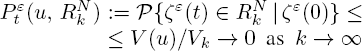
for all enough small ε > 0.
But by the property of stationary distribution one has:
Therefore, there exists a convergent sequence
We have to establish now that the measure π0(du) is a stationary distribution of the limit diffusion process, defined by generator [3.49].
Let ![]() be the transition probabilities of the limit diffusion process defined by generator [3.49].
be the transition probabilities of the limit diffusion process defined by generator [3.49].
According to theorem 3.2, the convergence
takes place uniformly for t ∈ [0, T] for any finite function ![]() with compact support. Consider a measure defined as
with compact support. Consider a measure defined as
and the functional
The convergence [3.56] implies the following limit representation:

Now we calculate
Using the relative compactness of the densities πε(du), ε > 0, established above, we get by [3.55] and [3.57] the following relations:
and by [3.58]
Putting the last two limits together, we obtain
It follows that

Hence, π0(dz) is the stationary measure of the limit diffusion process, defined by the limit generator [3.49]. The proofof theorem 3.3 is completed.
The construction of Lyapunov function V(u) can also be realized in another way.
Let us consider the limit diffusion process, defined by generators [3.37]-[3.39] with a constant covariance matrix and linear drift function with respect to u. Such a limit diffusion process is used in numerous applications.
LEMMA 3.2.- A diffusion process on real line R has the generator
where the drift function has the following form:
Then the Lyapunov function for the generator [3.59] can be chosen as follows:
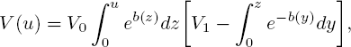
where the constants V0 > 0 and V1 satisfy the inequality
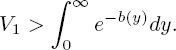
Here
PROOF.– (Proof of Lemma 3.2). Note that the integral in right-hand side of [3.62] is finite due to assumptions [3.60] and [3.63]. Using the first and second derivatives of the function [3.61], it is easy to calculate
Hence, the function V(u), given by [3.61], is excessive for the generator [3.59].
3.4. Markov queueing systems
There are two possibilities to construct diffusion approximations for real stochastic systems. Either to apply directly the pattern limit theorem 3.2 to a real queueing system and, then, compute local characteristics of the limit diffusion process by formulas [3.36], or to formulate some intermediate algorithm for a certain class of queueing systems. The second way is chosen.
3.4.1. Collective limit theorem in R1
Consider a normalized queueing process
where the queueing process νε(t) determines the number of customers in the system including that which have to be served at time t.
The positive valued centering function ρ(t),t ≥ 0,is supposed to be continuously differentiable. For simplicity, assume that the customers arrive and leave the system one by one.
The basic assumption is that the intensities of input and service times, under the condition νε(t) = k, depend on the parameter k in the following way:

with some given functions λ(v), μ(v), λ1(v) and μ1(v), v ∈ R1.
Note that the connection between the variables k = νε(t),v = ρ(t) and u = ζε(t) is represented as follows:
Therefore, the intensities of jumps of Markov process [3.64], under the condition ζε(t) = u, have the following representation:
THEOREM 3.4.– (Collective limit theorem). Let the intensities of input and service times of the queueing process νε(t) be set by relations [3.65]-[3.66] with continuously differentiable functions λ(u) and μ(u), having a bounded first derivative, and continuous functions λ1(u) and μ1(u). Let there exist a positive solution of evolutional equation
with initial condition ρ(0) = ρ 0 ≥ 0. And let the initial value of the queueing process converge, in probability, as follows:
Then the normalized queueing process [3.64] converges weakly as ε → 0 to a diffusion process ![]() :
:
The generator of the limit diffusion process ζ0(t) is determined by the relation:
where
The initial condition is ζ0(0) = ζ0.
PROOF.– (Proof of theorem 3.4). First, we calculate the local characteristics of the coupled Markov process ζε(t), ρ(t), t ≥ 0, using the representation [3.66] of jump intensities and the formulas [3.27] and [3.28]. The jump intensities [3.66] are transformed as follows:
with residual negligible terms θε(v, u) satisfying the condition [3.29]. By formulas [3.27], [3.35] and [3.36], we obtain
By formula [3.28], we get
At last, by balance condition [3.31]
We finish the proof of theorem 5.4 by applying theorem 3.2.
NOTE 3.3.- In the stationary regime with equilibrium point ρ:
the limit diffusion process is of the Ornstein-Uhlenbeck type with generator
where
The diffusion approximation algorithm of Markov queueing systems is formulated in the collective limit theorem 3.4. Under given intensities of input and service times represented in the form [3.65], the centered function ρ(t) is determined by a solution of evolutional equation [3.67] with velocity function, defined by [3.68]. The generator of the limit diffusion is defined by [3.70] with drift function given by [3.71] and covariance function given by [3.72]. The initial value of the limit diffusion is defined by [3.69].
3.4.2. Systems of M/M type
A single queueing system with unbounded queue is defined by input intensity λ and service time μ having exponential distributions.
COROLLARY 3.4.- Under the condition of heavy traffic λ > μ, the normalized queueing process
with centering function
where ρ0 is determined under the condition
converges weakly to a diffusion process ζ0 with zero mean and variance
COROLLARY 3.5.- An unbounded queueing system, with the rate of Poisson arrivals λ and the intensity of exponential distributed service time μ, has M/M/∞ type. The normalized queueing process [3.75] with centering function
where ρ0 is determined by initial condition [3.76] and converges weakly, as ε → 0,to a diffusion process ![]() , is defined by generator [3.70] with drift function
, is defined by generator [3.70] with drift function
and variance
3.4.3. Repairman problem
An extensive literature is devoted to this problem, for example, Iglehart (1965). There are n identical working devices that operate independently, m spare devices and r repairing facilities. If one of n operating devices fails, it transfers to a repair facility, being replaced by one of the spare devices. There are at most n devices operating at any time.
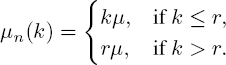
The working time of every device has exponential distribution with intensity λ. If r , or more, devices are being repaired, the failed device has to join a queue at the repair facility and wait for service. Let νn(t) be a number of devices undergoing or waiting for repair at a time instant t.
The diffusion approximation of queueing process νn(t) in the repairman problem depends on the correlations between parameters n, m and r.
There are considered to be three different variants.
COROLLARY 3.6.- (Iglehart (1965)). Let the following condition be fulfilled:
where m0 and r0 are fixed numbers and, in addition,
Then the normalized queueing process
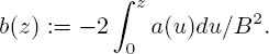
with centering constant
converges weakly, as n → ∞, to a diffusion process ζ0(t) with drift function a(u) = −uλ and variance B = 2r0μ.
PROOF.– A normalized queueing process can be represented as follows:
where κn(t) := νn(t)/n. This scaled process satisfies the inequality
The intensities of jumps of queueing process νn(t) are different on the intervals
namely

and
According to basic assumption [3.65] of theorem 3.4, the intensity functions are transformed to the next expression (considering the substitution ![]()

and

By assumptions [3.80] and [3.81] of corollary 3.6 and taking into account the condition
the normalized correlation has the form
Therefore, the intensity functions are considered on the intervals

and

The condition [3.80] of corollary 3.6 specifies the intensity functions on the interval
that is
Now, by theorem 3.4, we calculate the parameters of the limit diffusion:
with drift function
and variance
3.5. Markov queueing networks
3.5.1. Collective limit theorems in RN
A Markov network is determined by a finite number N of nodes. In every node there is a Markov queueing system. The customers are transferred from one node to another according to the marching matrix:
where pkr is probability of a custom transference from kth node to rth node.
The queueing process
is a vector function with components νk(t) of customers in kth node at time instant t. So the queueing process ν(t) takes values in the Euclidean space RN of the dimension N.
Consider an open network that means there exists at least one k for which
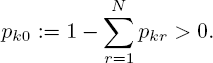
In other words, a customer leaves the kth node with probability pk0. The network temporal evolution is determined by intensity vector functions λ(u) = λk (u); 1 ≤ k ≤ N and μ(u) = μk(u); 1 ≤ k ≤ N where u = (uk): 1 ≤ k ≤ N) ∈ N. The customers arrive from outside at the kth node with exponentially distributed time intensity λk(u), and the exponentially distributed time of service at the kth node with intensity μk(u), 1 ≤ k ≤ N. Without loss of generality, assume that the virtual passages are not possible: pkk = 0 for all k. The diffusion approximation of queueing process begins by introduction of a small series parameter ε > 0. The main assumption is that the intensity functions depend on ε in the following form:
where u=(un; 1 ≤ n ≤ N) is a vector of values of the queueing process ν(t). The normalized queueing process is considered in a similar form as for the queueing system
with some deterministic positive-valued vector function
We use the following notation. A vector with the superscript “d” is a diagonal matrix, for example:
where δkr = 0, if k ≠ r, and δkk = 1 are Kronecker symbols.
THEOREM 3.5.– (Collective). Assume the following conditions:
- a) the vector functions λ(u) and μ(u) are continuously differentiable with bounded first derivatives;
- b) there exists a unique positive solution of differential equation
where
- c) the marching matrix P = [pkr ; 1 ≤ k, r ≤ N] is irreducible and invertible;
- d) the initial values of the normalized queueing process converge in probability: ζε(0) ⇒ ζ0 as ε → 0.
Then the normalized queueing process converges in probability
The limit ornstein-Uhlenbeck diffusion process ζ0(t), t ≥ 0 is defined by generator
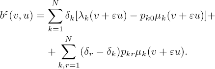
The covariance matrix B (u) is determined as follows:
where
PROOF._ (Proof of theorem 3.5). First of all, it is necessary to calculate the intensities of transfers of the normalized queueing process ζε(t). Let us introduce the notation
where δkr is the Kronecker symbol. Note that the normalized form of queueing process [3.85] determines the following relation between the variables ![]() and u = ζε(t):
and u = ζε(t):
Now it is possible to determine the jump intensities of the normalized Markov queueing process ζε(t):

The first formula gives the intensity of increase by one of the kth components νk(t): a customer arrives at the kth node of the network.
The second formula gives the intensity of decrease by one of the kth components νk(t): a customer leaves the network.
The third formula gives the intensity of increase by one of rth the components νr(t) and decrease by one of the kth components: a customer transfers from the kth node to the rth node of the network.
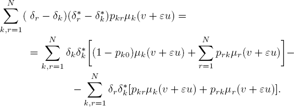
So the first two moments of jumps of the normalized queueing process [3.85] can be calculated. Using formula [3.27], the first moment in the following form is obtained:
Transforming the second term, one has

So the first moment has the following representation:

or, using notation [3.87], in the vector form:
Using Taylor’s formula, the asymptotic representation of the first moment is:
where ∣∣θε(v,u)∣∣ → 0 as ε → 0.
Hence, according to the notation in [3.27],
By theorem 3.2, it can be concluded that the centering function ρ(t) is determined by the solution of equation [3.86] and the drift function of the limit diffusion process is b(v, u) = u ∗ c′(v). The second moment of jumps of the normalized queueing process [3.85] with intensities of jumps [3.90] is calculated in a more complicated way. Using formula [3.28]

The second term is transformed as follows:
So the second moment has the following form:

or, using notation [3.89], the second moment is:
Applying the Taylor formula, it is seen that asymptotic representation of the second moment has the following expression:
Using theorem 3.2, the covariance matrix of the limit diffusion process is defined by relation >[3.89]. The proof of theorem 3.5 is completed.□
3.5.2. Markov queueing networks
Two types of Markov queueing networks and a superposition of independent Markov processes on a finite-dimensional phase state space are considered.
Network of [M |M| ∞]N type: the Markov queueing systems of type M ∣M ∣∞ are considered in each of N nodes of the network. Let the intensities of arrival times at the nodes of the network be determined by a vector λ(u) = (λk ; 1 ≤ k ≤ N) and let the intensities of service times in nodes of the network be determined by a vector μ(u) = (μk 1 ≤ k ≤ N).
COROLLARY 3.7.– The normalized queueing process of a network of [M ∣ M∣ ∞]N type
with the centering function is determined by the solution of the equation
where
under the conditions (c) and (d) of theorem 3.5 weakly converges as ε → 0 to an Ornstein–Uhlenbeck diffusion process with drift function
and covariance matrix
PROOF.˗ For the network of [M | M∣ ∞]N type, the intensity functions λ(u) and μ(u) in theorem 3.5 are determined as follows:
So, by formulas [3.86], [3.87], [3.91] and [3.92] one obtains [3.93] and [3.94], taking into account [3.88] and >[3.89]. □
Network of [M | M | 1| ∞]N type: the Markov queueing systems of M | M ∣1∣ ∞ type with intensities of arrival times λk and service times μk, 1 ≤ k ≤ M, are located in the nodes of the network.
COROLLARY 3.8.˗ The normalized queueing process of [M | M|∞]N type network
with centering function ρ(t) = ρ0 + Ct, C = λ + μ∗Q, where Q := [P − I], weakly converges, as ε → 0, to a diffusion process with zero mean and covariance matrix
PROOF.˗ By theorem 3.5, using the intensity vector function
according to formulas [3.86] and [3.87], the equation for the centered function is
Hence, the centering function is determined as ρ(t) = ρ0 + Ct. By formulas [3.88] and >[3.89], we can conclude that the drift function of the limit diffusion process is identically equal to zero, and the covariance matrix is given by [3.95]. □
3.5.3. Superposition of Markov processes
There are n independent ergodic Markov processes κi(t), 1 ≤ i ≤ n on a finite state space {0, 1,..., N } with generator matrix
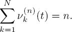
Introduce the counting process:
with components ![]() , which describe the number of Markov processes κi(t), 1 ≤ i ≤ n in the state (k , 1 ≤ k ≤ N). Let ρ =(ρk, 1 ≤ k ≤ N) be the stationary distribution of Markov processes:
, which describe the number of Markov processes κi(t), 1 ≤ i ≤ n in the state (k , 1 ≤ k ≤ N). Let ρ =(ρk, 1 ≤ k ≤ N) be the stationary distribution of Markov processes:

Introduce the notations:

COROLLARY 3.9.˗ The normalized counting process
weakly converges, as n →∞, to an Ornstein–Uhlenbeck diffusion process with drift function
and covariance matrix
PROOF.˗ The counting process [3.96] can be considered as a normalized queueing process for a Markov network with marching matrix

Consider the normalized counting process [3.96] in the following form:
Note that
Hence, the following relation exists between the two variables u = ζ(n)(t) and κ = K(n)(t):
or
Besides, ![]() , i.e.
, i.e. ![]() . Now determine the intensities of jumps of Markov process [3.96] under the condition
. Now determine the intensities of jumps of Markov process [3.96] under the condition
We leave it to the readers to complete the proof of corollary 3.9 similarly as in the proof of theorem 3.5.
3.6. Semi–Markov queueing systems
As indicated in the Introduction, the main problem is to choose an adequate method for asymptotic analysis of queueing processes in diffusion approximation schemes.
We will assume that the initial queueing process, scaled by a small series parameter ε → 0 (ε > 0), is set in the same way as in the Markov case:
However, now for simplicity, the centering constant ρ > 0 sets the equilibrium of the system evolution rate
The parameter

sets the average intensity of input flow of claims with a distribution function of intervals between the adjacent arrivals
The parameter μ > 0 determines the intensity of the claims service in the system, which have an exponential distribution of service intervals.
For simplicity, we consider a semi-Markov queueing system of S M | M | ∞ type. It means that the claims in the system are characterized by distribution function [3.100] with average intensity λ = 1/g, g := Eθn+1, n ≥ 0.
The intensity μ > 0 defines the exponential distribution of the claims processing time. The symbol “∞” means that the queueing system has an unbounded stock of claims.
The general scheme of asymptotic analysis of queueing systems is based on a compensating operator determined by the extended Markov process
Note the following property:
Hence the extended Markov process [3.101] is defined by the conditional distributions of increments
under the condition
The compensating operator of the extended Markov process [3.101] is determined as follows:
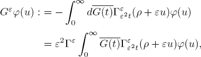
where the semigroup ![]() is defined by generator
is defined by generator
The asymptotic analysis of the compensating operator of the extended Markov process [3.105], as ε → 0 (ε >0), is given in the next theorem.
THEOREM 3.6.˗ Assume the following conditions:
- 1) the intensity of input claims λ = 1/g is bounded and λ > 0;
- 2) the accelerated intensity of service time με := μ ∕ ε > 0;
- 3) there exists the average limit
where the equilibrium ρ > 0 is determined by a balance condition for the velocity function
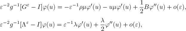
Then there exists a limit generator L0:
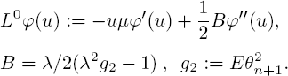
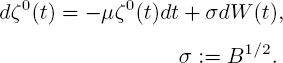
COROLLARY 3.10.˗The normalized compensating operator [3.101] weakly converges to a diffusion Ornstein˗Uhlenbeck process ![]() :
:
with generator [3.107], that is
PROOF. – (Proof of theorem 3.6). The following identity is used:
We use the following asymptotic representations of the terms in [3.111]:
and also
Therefore, the following representation takes place:
with a negligible term
More general models of semi-Markov queueing systems are considered in the previous study by Korolyk et al. (2008).
3.7. Acknowledgements
The authors warmly thank Prof. V.V. Anisimov for his kind invitation to participate in the book.
3.8. References
Anisimov, V.V. (1995). Switching processes: Averaging principle, diffusion approximation and applications. Acta Appl. Math. 40(2), 95–141.
Anisimov, V.V. (2002). Diffusion approximation in overloaded switching queueing models. Queueing Systems, 40, 141–180.
Anisimov, V.V. (2008). Switching Processes in Queueing Models. ISTE Ltd, London and John Wiley & Sons, New York.
Ethier, S.N., Kurtz, T.G. (1986). Markov Processes: Characterization and Convergence. Wiley, Hoboken.
Iglehart, D.L. (1965). Limit diffusion approximation for many-server queue and the repairman problem. J. Appl. Prob. 2, 429–441.
Korolyk, V.S., Mishkoy, G.H., Mamonova, A., Griza, I. (2008). Queueing system evolution in phase merging scheme. Buletinul Academiei De Stiinte a Republicii Moldova. Matematica 3(58), 83–88.
Korolyuk, V.S., Korolyuk, V.V. (1999). Stochastic Models of Systems. Kluwer, Dodrecht.
Korolyuk, V.S., Limnios, N. (2005). Stochastic Systems in Merging Phase Space. World Scientific, London.