
8
Recent Results in Finite-source Retrial Queues with Collisions
Anatoly NAZAROV1, Janos SZTRIK2 and Anna KVACH1
1National Research Tomsk State University, Russia
2University of Debrecen, Hungary
The aim of this chapter is to give a review of recent results on single-server finite-source retrial queueing systems with collision of the customers. These include investigations of when the server is reliable and models of when the server is subject to random breakdowns and repairs depending on whether it is idle or busy. Tool-supported, numerical, simulation and asymptotic methods are considered under the condition of unlimited growing number of sources. Several cases and examples are treated and the results of different approaches are compared to each other showing the advantages and disadvantages of the given method. In general, we prove that the steady-state distribution of the number of customers in the service facility can be approximated by a normal distribution with given mean and variance. Using asymptotic methods under certain conditions in steady state, the distribution of the sojourn time in the orbit and in the system can be approximated by a generalized exponential one. Furthermore, it is proved that the distribution of the number of retrials until the successful service in the limit is geometrically distributed. With the help of stochastic simulation, several systems are analyzed showing directions for further analytic investigations. Tables and figures are presented to illustrate some special features of these systems.
8.1. Introduction
Finite-source retrial queues are very useful and effective stochastic systems to model several problems arising in telephone switching systems and telecommunication networks including cellular networks, CSMA (carrier sense multiple access) local area computer networks, call centers and CSMA-based wireless mesh networks at the frame level. To see their importance, the interested reader is referred to the following work and references cited in them: Artalejo and Corral (2008); Falin and Artalejo (1998); Fiems and Phung-Duc (2017); Gómez-Corral and Phung-Duc (2016); Kim and Kim (2016).
Searching the scientific databases, we have noticed that just a relatively small number of papers have been devoted to queueing systems when the arriving calls (primary or secondary) cause collisions to the request under service and both go to the orbit (see, for example, Ali and Wei (2015); Choi et al. (1992); Kim (2010); Kumar et al. (2010); Lakaour et al. (2018); Peng et al. (2014); Takeda and Yoshihiro (2017)).
In real CSMA systems, collisions are unavoidable and they decrease the effectiveness of the system performance and that is why new protocols should be developed to avoid them (see Cao et al. (2018); Jinsoo et al. (2018); Kwak et al. (2018); Wentink (2017); Yeo et al. (2017)). Real situations where collisions may occur were modeled by Reith (2017) and Takeda and Yoshihiro (2017).
Stochastic modeling of systems with collisions is required not only from a technical point of view but it is a mathematical challenge since it needs more sophisticated approaches.
Nazarov and his research group developed a very effective asymptotic method (Nazarov and Moiseeva 2006) with the help of which various systems have been investigated. Concerning finite-source retrial systems with collision, we should mention the following papers: Kvach and Nazarov (2015b); Kvach (2014); Kvach and Nazarov (2015a,c); Nazarov et al. (2014).
Sztrik and his research group have been dealing with systems with unreliable server/s as can be seen in Almási et al. (2005); Sztrik (2005); Sztrik et al. (2006); Wuchner et al. (2010) and that is why it was understandable that the two research groups started cooperation in 2017.
Our investigations have been based on analytical, numerical, simulation and asymptotic approaches as treated in Anisimov and Sztrik (1989); Anisimov and Artalejo (2001); Anisimov (1999); Artalejo and Corral (2008); Bhat (2015); Bossel (2013); Falin and Templeton (1997); Harchol-Balter (2013); Kobayashi and Mark (2009); Kulkarni (2016); Lakatos et al. (2013); Law and Kelton (1991); Nazarov and Terpugov (2004); Nazarov and Moiseeva (2006); Rubinstein and Kroese (2016); Stewart (2009); Yao (2016).
The primary aim of this chapter is to give a survey on the results obtained in this field in the recent past by means of different methods. Doing so we have tried to unify the notation which has appeared in different publications and to use the standard notation of Western-style papers, which differs from the Russian-style papers. We are confident that our models with collision can be used in real situations to describe, for example, the operation of random access systems treated in Fiems and Phung-Duc (2017) without collision; CSMA-based wireless mesh networks at frame and packet level investigated in Takeda and Yoshihiro (2017); and systems with transmission errors analyzed in Lakaour et al. (2018). When a collision occurs, signals are superimposed, packets are distorted and therefore packets need to be retransmitted, for which they both should be sent to the orbit.
We agree that the light-traffic approach applied in Fiems and Phung-Duc (2017) to get the distribution of the number of customers in the service facility for systems without collisions could be integrated to investigate systems with collisions. However, we must emphasize that beside these we are able to obtain approximation for the distribution of a number of retrials and for the distribution of the response/waiting time of a customer. These measures were not treated in the above-mentioned paper. In addition, in our different cases the service time is generally distributed and the server is not reliable.
From the theoretical point of view, one of the main difficulties compared to the systems without collision is that the service process is interrupted many times by the collisions until it is successfully completed. Unreliable server failures also interrupt the service, resulting in a quite complicated total service time structure. In addition, in case of a collision the number of customers in the orbit increases by two. Using an algorithmic approach means that the nth iteration depends on not only the previous iteration but on two previous ones. Our most important contribution is that, besides obtaining the asymptotic distribution of the number of customers in the orbit, the asymptotic distribution of the number of retrials and the distribution of the response/waiting time of a call are determined under certain conditions.
The new numerical insights for models with collisions and unreliable server are obtained by the help of algorithmic, numeric (MOSEL), simulation approaches. The combination of these methods allows us to validate the accuracy of the asymptotic method. We show that under a certain parameter setup, the characteristic property of the finite-source retrial queues having a maximum of the mean waiting time for an increasing arrival rate remains valid even in case of collision. This means that the maximum is due to the finite source and not to the collision. This surprising feature was noticed by several authors and it was explained in several ways. However, in systems with collisions we have to deal with the total service time, which is many times interrupted by collisions and failures. This notion is due to the collision and the successful service time is the last phase of this measures of interest. According to our experiments, the mean of the total and successful service time heavily depends on the distribution of the service time and the minimum can be obtained only under very special parameter setup.
This chapter is an enlarged and modified version of our recent paper (Nazarov et al. 2018).
The rest of the paper is organized as follows. In section 8.2, a description of the model is given, and the corresponding multi-dimensional non-Markov process is defined. In sections 8.3 and 8.4, systems with a reliable and an unreliable server are treated, respectively. In these sections, models with exponentially and generally distributed service times are investigated, and then analyzed by means of tool supported, algorithmic, simulation and asymptotic methods, respectively. The main results of the papers are collected and several figures illustrate the most interesting features of the given system. Finally, this chapter ends with a conclusion and some future plans are highlighted.
8.2. Model description and notations
In the following, we introduce the model in the most general form as it was treated with the help of numerical and asymptotic methods.
Let us consider a retrial queuing system of type M/GI/1//N with collision of the customers and an unreliable server (Figure 8.1). The number of sources is N and each of them can generate a primary request during an exponentially distributed time with rate λ/N. A source cannot generate a new call until the end of the successful service of this customer.

Figure 8.1. Retrial queuing system of type M/GI/1//N with collisions of the customers and unreliable server
If a primary request finds the server idle, he enters into service immediately, in which the required service time has a probability distribution function B(x). Let us denote its service rate function by μ(y) = B’ (y)(1 − B(y))−1 and its Laplace -Stieltjes transform by B*(y), respectively. If the server is busy, an arriving (primary or repeated) customer goes into collision with a customer under service and they both move into the orbit. The interretrial times of customers are supposed to be exponentially distributed with rate σ/N, that is, it does not depend on how many times it has been blocked. We assume that the server is unreliable, that is its lifetime is supposed to be exponentially distributed with failure rate γ0 if the server is idle and with rate γ1 if it is busy. When the server breaks down, it is immediately sent for repair and the repair time is assumed to be exponentially distributed with rate γ2. We deal with the case when the server is down, all sources continue generation of customers and send them to the orbit; similarly, customers may retry from the orbit to the server but all arriving customers immediately go into the orbit. Furthermore, in this unreliable model, we suppose that the interrupted request goes to the orbit immediately and its next service is independent of the interrupted one. Of course, in the case of a reliable server γ0 = γ1 = 0. All random variables involved in the model construction are assumed to be independent of each other.
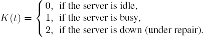
Let J(t) be the number of customers in the system at time t, that is, the total number of customers in the orbit and in service. Similarly, let K(t) be the server state at time t, that is
Thus, we will investigate the process {K(t), J(t)}, which is not a Markov process unless the service time is exponentially distributed. To be a Markov process we must use the method of supplementary variables, namely, we will consider two variants: the residual service time method and the elapsed service time method depending on what the aim of the investigation is.
Let us denote by Y(t) the supplementary random process equals the elapsed service time of the customer till the moment t and by Z(t) the residual service time, that is, the time interval from the moment t until the end of successful service of the customer, respectively. It is obvious that {K(t), J(t), Y(t)} and {K(t), J(t), Z(t)} are Markov processes. Let us note that Y (t) and Z(t) are defined only in those moments when the server is busy, that is, when K(t) = 1.
Let us define the stationary probabilities as follows:

Of course, in the case of exponentially distributed service time the steady-state probabilities are denoted as follows:
The steady-state distribution of the server’s state is denoted by
and the distribution of the number of customers in the system is designated by
It is clear that in the case of a reliable server, all the probabilities where K = 2 are 0.
The main aim of the investigations is to get these distributions and other performance measures of the systems, such as the distribution of the sojourn time in the system, distribution of the total service time and distribution of the number of retrials. These are very complicated problems and to the best knowledge of the authors there are no exact analytical formulas to the solutions. That is the reason we have tried to obtain the characteristics of different systems by the help of tool supported, algorithmic, stochastic simulation and asymptotic methods.
Since in the following, we will use the gamma distribution to show special features of some systems we introduce it here to be sure of the form because it is defined in several ways.
A random variable X is said to have a gamma distribution with parameters (α,β) if its density function is given by
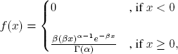
where α > 0, β > 0, and
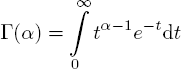
is the so-called complete gamma function.
Its distribution function cannot be obtained in an explicit form except α = n. In this case, it reduces to the Erlang distribution.
It should be noted that depending on the parameters it can take small values with high probability, that is when the shape parameter is low, in this case the squared coefficient of variation ![]() is high. Its density function has the form
is high. Its density function has the form
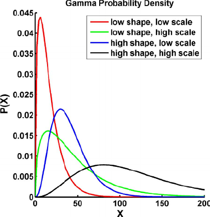
Figure 8.2. Density function of the gamma distribution. For a color version of this figure, see www.iste.co.uk/anisimov/queueing1.zip
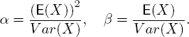
It can be shown that
α and β are called the shape parameter and scale parameter, respectively, and they can be expressed by the mean and variance in the following way if we would like to estimate the parameters from the sample
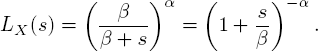
It can be shown that its Laplace transform has the form
8.3. Systems with a reliable server
8.3.1. M/M/1 systems
8.3.1.1. Algorithmic approach
In previous papers (Kvach 2014; Nazarov et al. 2014), the steady-state Kolmogorov equations were derived and the distribution of the system’s state was obtained by an algorithmic approach. Then the distribution of the number of customers in the system were calculated and used to validate the asymptotic results.
8.3.1.2. Asymptotic approach
The main contribution of the paper by Nazarov et al. (2014) is that the steady-state characteristic function of prelimit distribution of the number of customers in the system can be approximated by the following third-order asymptotic characteristic function, that is

where the distribution of the server’s state is explicitly given in the following form:

and the cumulants (semi-invariants) (Nazarov and Sudyko 2010) are
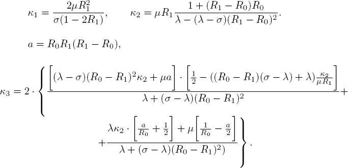
Actually, κ1 is the positive solution of the equation
and numerically it is easy to verify that
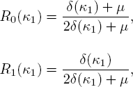
where δ(κ1) = λ(1 − κ1) + σκ1.
It is easy to see that the second-order approximation results in a normal distribution. In this case, let us denote by G(x) the distribution function of the Gaussian distribution with mean Nκ1 and variance Nκ2.
Furthermore, let us denote by Pas(j) the asymptotic discrete distribution obtained by the help of Gaussian approximation, that is

which we will call the Gaussian approximation of the prelimit discrete distribution P(j).
In the following, we show how we can get the distribution with the help of the inverse characteristic function (see Nazarov and Sudyko (2010)).
Let Dm(j) be a probability distribution with j = 0, 1, 2, ..., N and hm(u) its characteristic function, that is

where i = ![]() is the imaginary unit and hm(u) is the mth-order asymptotic characteristic function. Then using the inverse transformation Dm(j) is given by the formula
is the imaginary unit and hm(u) is the mth-order asymptotic characteristic function. Then using the inverse transformation Dm(j) is given by the formula
It is obvious that
If the values of Dm(j) are real and non-negative for all j = 0,...,N, then
where Pm(j) is called the mth-order approximation of the prelimit distribution P(j).
Since Dm(j) is calculated by numeric integration, among the numbers Dm(j) there can appear complex numbers with small enough imaginary parts or real negative numbers with small enough absolute values.
In this case, we define real non-negative numbers gm(j) by the formula
where the over bar denotes complex conjugation. Then let us define the approximation of the prelimit distribution by the equality
To compare the probability distributions P(j) and Pm(j), we will use the Kolmogorov distance defined as
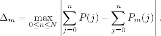
By this distance, we can estimate the error of the mth-order approximation of the prelimit distribution.
In a previous paper (Nazarov et al. 2014), second- and third-order approximations of the prelimit distribution were compared to the exact distribution obtained by the algorithmic method. With a different parameter setup and for different N, the applicability of the asymptotic method was validated and some conclusions were drawn.
A more complicated problem, namely the distribution of the sojourn time in the service facility, was investigated by Kvach and Nazarov (2015b) with the help of asymptotic methods as N tends to infinity. It was proved that the characteristic function of the sojourn time T that a customer spends in the service facility can be approximated by
where ![]() .
.
Then it is easy to show that the approximation of the prelimit distribution function of the sojourn time can be written as
which means that the asymptotic sojourn time can be zero with probability q and it is exponentially distributed with probability 1− q. As a result, the mean sojourn time
From probabilistic reasoning
which means that the mean arrival rate is equal to the mean departure rate and from Little’s formula
should be valid. These formulas can be used for validation of the obtained numerical and asymptotic results. The asymptotic sample examples concerning the sojourn time distribution have not been validated by simulation in the paper.
8.3.2. M/GI/1 system
This section deals with the results when the required service times are generally distributed but in the examples the gamma distribution is used due to its useful properties. Namely, it is easy to see that its squared coefficient of variation can be less, equal to or greater than 1 depending on the values of the shape and scale parameters.
8.3.2.1. Algorithmic approach
A previous study (Kvach and Nazarov 2015a) deals with the algorithmic approach of how to get the steady-state distribution of the system. The method of supplementary variable technique with residual service time were applied and several numerical examples were treated with gamma distributed service time. The results helped the validation of asymptotic results for the same model.
8.3.2.2. Stochastic simulation
Papers of Nazarov et al. (2017b,c) are devoted to the asymptotic analysis of the mean total service time, distribution of the sojourn time in the system and the distribution of the number of retrials. It must be noted that the results have not been validated by simulation. Meanwhile, simulations have been carried out, the estimations for the mean and variance of the sojourn time have been obtained, and the distribution of the number of retrials also has been determined. The simulation analysis will be published in the near future.
8.3.2.3. Asymptotic approach
In this section, the asymptotic results published in Nazarov et al. (2017b,c) are summarized. Before doing that we need some notations, namely
Then κ1 can be obtained from
and the distribution of the server’s state can be determined by
In the case of the residual service time until the successful service completion approach for the busy server’s sate, we have
and in the case of the elapsed service time approach we get

Introducing the notations
we obtain

Consequently, the steady-state prelimit distribution of the number of customers in the system can be approximated by a normal distribution with mean Nκ1and variance Nκ2.
It is interesting that equation [8.2] can have one, two or three roots 0 <κ1 < 1. For example, for the gamma distribution function B(x) with a shape parameter α and scale parameter β with values α = β = 2, λ = 0.29, σ = 20, equation [8.2] has three roots, namely ![]()
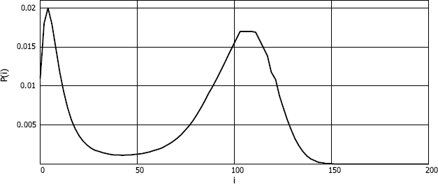
Figure 8.3. Bimodal probability distribution of the number of customers in the system
Let us consider such values of the service parameters α, β and the system λ, σ at which equation [8.2] has three roots; the probability distribution P(i) = P{i(t) = i} can then be of a bimodal type. In particular, for α = β = 2, λ = 0.29, σ = 19.7 by simulation and numerical methods at N = 200 for P(i) we obtain the following graph shown in Figure 8.3.
The reason for this feature is explained by Nazarov et al. (2017c).
As a rule, equation [8.2] has three roots in exceptional cases at special values of parameters and such situation arises extremely rare. Therefore, in the following let us consider some properties of the system when the main equation [8.2] has a single root 0 <κ1 < 1 .
In the paper by Nazarov et al. (2017b), for the mean sojourn time of the customer in service, we get the following expression:
Next let us consider the influence of the system parameters on the mean sojourn time E(TS) of the customer in the server. We will choose σ = 20 and the values of parameters λ and α = β are specified in Table 8.1
As we can see, at α < 1 the values of total mean sojourn time E(TS) of the customer under service takes values less than unity. For α < 1, there is a high probability of emergence of small values of service time and this fact undoubtedly influences the total mean sojourn time E(TS) of the customer at the server and it takes rather small values. Moreover, let us note that with increasing values of parameter λ the values of E(TS ) decrease.
Table 8.1. Mean sojourn time E(TS) of the customer under service at various values of λ and α = β
| α = β | |||||||||
|---|---|---|---|---|---|---|---|---|---|
| 0.1 | 0.3 | 0.5 | 0.8 | 1 | 2 | 3 | 5 | ||
| 0.5 | 0.324 | 0.546 | 0.682 | 0.857 | 1 | 5.038 | 20.816 | 153.239 | |
| 1 | 0.204 | 0.367 | 0.488 | 0.727 | 1 | 5.576 | 21.695 | 154.766 | |
| λ | 5 | 0.067 | 0.165 | 0.301 | 0.640 | 1 | 5.937 | 22.360 | 155.975 |
| 10 | 0.046 | 0.140 | 0.280 | 0.632 | 1 | 5.979 | 22.441 | 156.125 | |
| 15 | 0.039 | 0.131 | 0.273 | 0.629 | 1 | 5.993 | 22.468 | 156.175 | |
In the case of α > 1, the values of E(TS) become greater than unity. Table 8.1 illustrates that with an increase of service parameter α the values of total mean sojourn time E(TS) of the customer under service considerably increases and reaches very large values. Let us note that in this situation, parameter λ practically does not influence E(TS) and with an increasing parameter of service α this influence becomes less and less.
Table 8.1 also shows that in case of exponential service time, i.e. α = β = 1, the values of total mean sojourn time E(TS ) of the customer at the server are equal to the unit.
For the distribution of the number of retrials/transitions of the tagged customer into the orbit, we have the following results.
Let ν be the number of transitions of the tagged customer into the orbit, then
where value of parameter q has a form
From the proved theorem, it obviously follows that the probability distribution P {ν = n} , ![]() of the number of transitions of the tagged customer into the orbit is geometric and
of the number of transitions of the tagged customer into the orbit is geometric and
Consequently, by using the law of total probability for the characteristic function of the sojourn/waiting time W of the tagged customer in the orbit we get
In the case of N → ∞, the limiting probability distributions of the sojourn time of the customer in the system T and the sojourn time of the customer in the orbit W coincide, namely
Let us consider the influence of the system parameters on the values of the mean number of retrials ν . We will choose the same system parameters which have been considered in the previous examples, namely σ = 20, and the values of parameters λ and α =β , are specified in Table 8.2.
Table 8.2. Mean number of retrials for various values of λ and α = β
| α = β | |||||||||
|---|---|---|---|---|---|---|---|---|---|
| 0.1 | 0.3 | 0.5 | 0.8 | 1 | 2 | 3 | 5 | ||
| 0.5 | 0.470 | 1.131 | 1.86 | 3.65 | 6.32 | 162.7 | 793 | 6091 | |
| 1 | 0.656 | 2.002 | 4.19 | 11.57 | 21.83 | 204.1 | 848 | 6172 | |
| λ | 5 | 1.114 | 4.192 | 9.31 | 22.73 | 37.07 | 234.4 | 891 | 6236 |
| 10 | 1.278 | 4.755 | 10.28 | 24.30 | 39.02 | 238.1 | 896 | 6244 | |
| 15 | 1.355 | 4.969 | 10.63 | 24.83 | 39.67 | 239.3 | 898 | 6247 | |
From Table 8.2, it is shown that the mean number of retrials obviously depends on service parameter α that is the expected and logical result. It should be noted that for small values of parameter α, the influence of parameter λ on the mean number of retrials is significant and obvious. But with the increase in parameter α, this influence decreases and already for great values of α practically disappears.
The following conclusions can be drawn: the mean number of retrials and mean sojourn time of the customer under service is a consequence of the collision of customers and the admissibility of repeated attempts of service by the same customer. Duration of the customer service for repeated attempts has the same probability distribution B(x), but its repeated realization, naturally, accepts various values. If for the distribution B(x), there is a high probability of emergence of small values of service time as in the gamma distribution with the shape parameter α < 1, then a small number of retries is sufficient to realize a small value of the service time which will be successful. If the small values of the service time are unlikely for the probability distribution B(x), as in the gamma distribution with the shape parameter α > 1 , then the number of unsuccessful attempts of service becomes big, as we can see in Table 8.2, the server works without results, the mean sojourn time of the customer under service increases (Table 8.1).
8.4. Systems with an unreliable server
In many practical situations, the server is not reliable and after a random time it can fail and needs repair which also takes a random duration. To deal with these service interruptions, several papers have been published (see, for example, Almási et al. (2005); Dragieva (2014); Gharbi and Dutheillet (2011); Gharbi and Ioualalen (2006); Gharbi et al. (2014); Krishnamoorthy et al. (2014); Roszik (2004); Sztrik et al. (2006); Wang et al. (2010, 2011); Zhang and Wang (2013)). In the following sections, we summarize our results obtained by different methods.
8.4.1. M/M/1 system
8.4.1.1. Tool-supported approach by MOSEL
Because of the fact that in many practical situations the state space of the describing Markov chain is very large, it is rather difficult to calculate the system measures in the traditional way of writing down and solving the underlying steady-state equations. To simplify this procedure, several software packages have been developed and effectively used for performance evaluation of complex systems (see, for example, Gharbi and Dutheillet (2011); Gharbi and Ioualalen (2006); Gharbi et al (2015); Gharbi et al. (2014); Ikhlef et al. (2016)). In our investigations, a similar software tool called MOSEL (Modeling, Specification and Evaluation Language) has been used to formulate the model and to obtain the performance measures. A previous study by Bérczes et al. (2017) deals with the model formulation, derivation of several performance measures and generation of illustrative examples showing an interesting phenomenon of finite-source retrial queues, that is under specific parameter setup the mean waiting/sojourn time has a maximum as the arrival intensity is increasing. We showed that it still remains in the case of collisions as the following example shows
| Case | N | λ/N | γo | γ1 | γ2 | σ/N | μ |
|---|---|---|---|---|---|---|---|
| Figure 8.4 case 1 | 100 | 0.01 | 0.01 | 0.01 | 1 | 0.1 | 1 |
| Figure 8.4 case 2 | 100 | 0.01 | 0.1 | 0.1 | 1 | 0.1 | 1 |
| Figure 8.4 case 3 | 100 | 0.01 | 1 | 1 | 1 | 0.1 | 1 |
| Figure 8.5 | 100 | 0.03-8.1 | 0.01 | 0.01 | 1 | 0.1 | 1 |
| Figure 8.6 | 100 | 0.03-8.1 | 0.1 | 0.1 | 1 | 0.1 | 1 |
Figure 8.4 shows the steady-state distribution of the three investigated cases. In this figure, we can see also the effect of the breakdown of the server. We can see that the mean number of customers increases as the breakdown intensity gets larger. From the shape of the curves, it is clearly visible that the steady-state distribution of the cases are normally distributed.
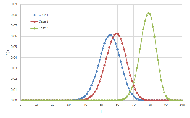
Figure 8.4. Steady-state distributions. For a color version of this figure, see www.iste.co.uk/anisimov/queueing1.zip
Figures 8.5 and 8.6 show the mean response time as a function of the customer generation rate. As we can see, the mean response time will be greater as we increase the generation rate, but after λ/N is greater than 1.5 the mean response time starts to decrease.
8.4.1.2. Algorithmic approach
The advantage of an algorithmic approach to the general tool supported method is that in this case we do not have a state space explosion and N can be much higher than in case of calculations carried by MOSEL as we will see soon. The publication of the results has been submitted (see Kuki et al. (2019)). The calculation has been performed by a spreadsheet program, MS Excel, and N can be arbitrary large. When the calculations are performed by the MOSEL-2 tool (see Bérczes et al. (2017)), we run into strict limitations, namely the state space grows extremely fast; consequently the number of sources cannot exceed 200. In Excel, we can go far higher above 200. Other advantages for using this spreadsheet are that the effect of parameter modifications can be seen immediately and the set of the steady-state probabilities, both the two- and one-dimensional ones, are present in separate columns and can be used directly for further investigations.

Figure 8.5. vs λ∕N, 
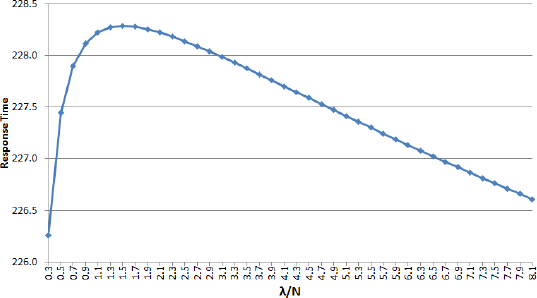
Figure 8.6. vs λ∕N,
For illustration, we consider three systems with the following input parameters
N = 100, λ= 1, μ= 1, σ= 5, γ0 = 0.1, γ1 = 0.1, γ2 = 1.
In Figure 8.7, the steady-state probabilities of three models are displayed: a basic reliable system with no conflict, a reliable system with conflict, and an unreliable system with conflict. In the no conflict case, the expectation of states are lower than for the other cases. The probabilities of the states have the greatest mean in the unreliable system as it was expected.
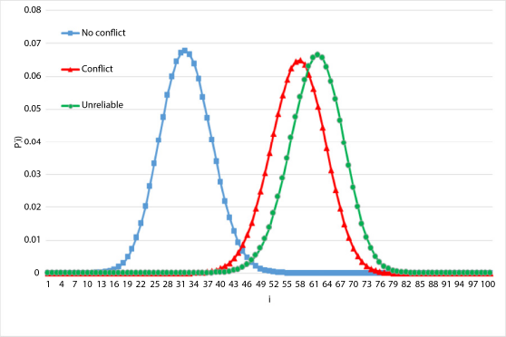
Figure 8.7. Reliable no conflict, reliable with conflict, and unreliable with conflict. For a color version of this figure, see www.iste.co.uk/anisimov/queueing1.zip
8.4.1.3. Stochastic simulation
To validate the applicability of the asymptotic approach, we need either numerical or simulation results. The correct operation of the simulation software was tested by the numerical sample examples. The investigations carried out by the simulation and asymptotic methods have been submitted for publication (see Nazarov, Sztrik, Kvach and Bérczes (2018) and Nazarov, Sztrik, Kvach and Tóth (2018)).
8.4.1.4. Asymptotic approach
First, we deal with the distribution of the number of customers in the system as it has been published by Nazarov et al. (2018). The first-order asymptotic results are the following
where κ1 is the positive solution of the equation
where the stationary distributions of probabilities Rk(κ1) of the server state k = 0, 1, 2 are obtained as follows

here a (κ1 ) is
The second order asymptotic results are

where κ2 is
and
Consequently, the prelimit distribution of the number of customers in the system can be approximated by a normal distribution with mean Nκ1 and variance Nκ2.
Let us determine the accuracy and area of applicability of this approximation.
We have the following input parameters:
and we will provide values of Kolmogorov distance Δ in Table 8.4.
Table 8.4. Kolmogorov distance between prelimit distribution P(i) and the asymptotic distribution Pas(i) for various values of the parameters N and λ
| N = 5 | N = 10 | N = 20 | N = 30 | N = 50 | |
|---|---|---|---|---|---|
| λ = 0.5 | 0.095 | 0.059 | 0.032 | 0.023 | 0.017 |
| λ = 1.0 | 0.037 | 0.023 | 0.017 | 0.014 | 0.011 |
| λ = 2.0 | 0.078 | 0.046 | 0.022 | 0.014 | 0.013 |
Table 8.5 demonstrates the Kolmogorov distance for the following parameters:
and for various values of the parameter N and σ.
Table 8.5. Kolmogorov distance between prelimit distribution P(i) and the asymptotic distribution Pas(i) for various values of the parameters N and σ
| N = 5 | N = 10 | N = 20 | N = 30 | N = 50 | |
|---|---|---|---|---|---|
| σ = 0.2 | 0.066 | 0.035 | 0.018 | 0.013 | 0.010 |
| σ = 1.0 | 0.033 | 0.018 | 0.014 | 0.014 | 0.008 |
| σ = 5.0 | 0.037 | 0.023 | 0.017 | 0.014 | 0.011 |
Assuming an acceptable error Δ ≤ 0.05 of the given values in Tables 8.4–8.5, we can conclude that approximation has a large error at N ≤ 10,at 10 < N < 20 the acceptability of approximation is doubtful, and at N ≥ 20 approximation has quite acceptable accuracy.
Let us turn our attention to the analysis of the waiting/sojourn time distribution. Using Little’s formula, we have
therefore
where κ1 is the asymptotic average value of the number of customers in the system, and (1 – κ1)λ is the mean arrival intensity of the incoming flow.
However, we should underline that the above equality [8.3] defines only the mean sojourn time of the customer in the system. We would like to carry out a more detailed investigation for T of the tagged customer.
One of the main contributions of Nazarov et al. (2018) is that for the limit of the characteristic function of the normalized sojourn time we have
where q is
Consequently, the characteristic function of the sojourn time of the customer in the system in the prelimit situation of finite N can be approximated by
In the following, let us find the average value of the normalized sojourn time of the customer in the system which is
and that coincides with the result earlier obtained by Little’s formula.
For the distribution of the number of transitions/retrials of the tagged customer into the orbit, we get the following results.
Let ν be the number of transitions of the tagged customer into the orbit, then
resulting in the probability distribution P {ν = n}, ![]() of the number of transitions of the tagged customer into the orbit being geometric and having the form
of the number of transitions of the tagged customer into the orbit being geometric and having the form
Consequently, the prelimit characteristic function of the sojourn/waiting time W of the tagged customer in an orbit can be approximated as
In the case of N → ∞, the limiting probability distributions of the sojourn time of the customer in the system T and the sojourn time of the customer in an orbit W coincide, namely
Previously, we have obtained that the probability distribution of the number of transitions of the tagged customer into the orbit is geometric with parameter q. Let us find out how close the limiting results to the simulation results and at what values N this approximation is admissible.
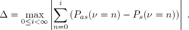
To do so, let us denote by Pas(ν = n) the asymptotic geometric distribution of probabilities with parameter q and by Ps (ν = n) the probability distribution of the number of transitions of the tagged customer into the orbit obtained with the help of simulation program. Furthermore, let us determine the accuracy (error) of approximation of distribution by mean of Kolmogorov distance Δ, which for probability distributions Pas(ν = n) and Ps(ν = n) is defined as
Realizing the simulation program for
and applying the approximation we will provide the Kolmogorov distance Δ for various values N and γ = γ0 = γ1 in Table 8.6.
We can see, as expected, that by increasing N the Kolmogorov distance should decrease, but with this parameter setup there is no essential reduction if N > 50.
Let us see the mean number of retrials under the same condition as before.
Again we can observe what was expected: as N increases the mean number of retrials increases since there are more and more customers in the system resulting in more and more collisions. At the same time, it can also be seen how the mean number of retrials increases as the failure rate of the server increases. It should be underlined that each time the limiting values give very good approximations showing the effectiveness of the asymptotic method.
Table 8.6. Kolmogorov distance between distribution Ps(i) and approximation of the geometric distribution Pas(i) for various values of the parameters N and γ
| N = 20 | N = 30 | N = 50 | N = 100 | N = 200 | |
|---|---|---|---|---|---|
| γ = 0.05 | 0.026 | 0.016 | 0.009 | 0.005 | 0.003 |
| γ = 0.1 | 0.024 | 0.015 | 0.009 | 0.004 | 0.002 |
| γ = 0.5 | 0.017 | 0.011 | 0.006 | 0.004 | 0.001 |
8.4.2. M/GI/1 system
8.4.2.1. Stochastic simulation
In Tóth et al. (2017), the required service time is supposed to be gamma distributed and the input parameters of the system are collected in Table 8.8.
Table 8.8. Numerical values of model parameters
| Case | N | λ/N | γ0 | γ1 | γ2 | σ / N | α | β |
|---|---|---|---|---|---|---|---|---|
| 1 | 100 | 0.01 | 0.1 | 0.1 | 1 | 0.01 | 0.5 | 0.5 |
| 2 | 100 | 0.01 | 0.1 | 0.1 | 1 | 0.01 | 1 | 1 |
| 3 | 100 | 0.01 | 0.1 | 0.1 | 1 | 0.01 | 2 | 2 |
Figure 8.8 shows the steady-state distribution of the three investigated cases. It is observed that the mean number of customers increases as α and β are getting larger. Case 2 is a special case because when α = 1, it represents the exponential distribution. From the shape of the curves, it is clearly visible that the steady-state distribution of the cases are normally distributed. The next table presents the considered performance measures in relation with the different cases (see Table 8.9).

Figure 8.8. Comparison of steady-state distributions. For a color version of this figure, see www.iste.co.uk/anisimov/queueing1.zip
In Table 8.9, the notations mean the followings: E(J) and Var(J) are mean number and variance of customers in the system, E(T) and Var(T) are mean and variance of response time, E(W) and Var(W) are mean and variance of waiting time, E(S) and Var(S) are mean and variance of successful service time, andE(IS) is mean interrupted service time.
Table 8.9. Simulation results
| Case | E(J) | Var(J) | E(T) | Var(T) | E(W) | Var(W) | E(S) | Var(S) | E(IS) |
|---|---|---|---|---|---|---|---|---|---|
| 1 | 63.6842 | 27.9734 | 175.3073 | 65, 657.3454 | 174.5884 | 65, 434.6696 | 0.3147 | 0.1979 | 0.4041 |
| 2 | 70.5912 | 24.3012 | 239.9734 | 105, 273.4267 | 238.9734 | 104, 918.6389 | 0.4784 | 0.2289 | 0.5217 |
| 3 | 75.1825 | 21.2439 | 302.8106 | 151, 781.1411 | 301.5377 | 151, 277.6006 | 0.6472 | 0.2095 | 0.6257 |
Figure 8.9 represents the confirmation of mean waiting time. The same parameters are (see Table 8.9) used as shown in Figure 8.8 but here the running parameter is λ/N. As is expected with the increment of λ ∕ N, mean waiting time increases as well but an interesting phenomenon is noticeable, namely that after λ ∕ N is greater than 0.1 mean waiting time starts to decrease.

Figure 8.9. Mean waiting time versus intensity of incoming customers. For a color version of this figure, see www.iste.co.uk/anisimov/queueing1.zip
8.4.2.2. Asymptotic approach
These results have been published by Nazarov et al. (2017a) using a supplementary variable technique. The limit of the characteristic function of the scaled number of customers in the systems can be written in the following form
where κ1 is the positive solution of the equation
here δ (κ1 ) is
and the stationary distributions of probabilities Rk(κ1) of the server’s state k = 0, 1, 2 are determined as follows:

8.4.3. Stochastic simulation of special systems
In Tóth et al. (2017), systems with not only gamma distributed service times but also gamma distributed interarrival and gamma distributed retrial times have been investigated.
8.4.3.1. Gamma distributed interarrival times
Table 8.10 presents the input parameters of this case.
Table 8.10. Numerical values of parameters of gamma distributed interarrival times
| Case | N | α | β | γ0 | γ1 | γ2 | σ / N | α1 | β1/N |
|---|---|---|---|---|---|---|---|---|---|
| 1 | 100 | 1 | 1 | 0.1 | 0.1 | 1 | 0.01 | 0.5 | 0.01 |
| 2 | 100 | 1 | 1 | 0.1 | 0.1 | 1 | 0.01 | 1 | 0.01 |
| 3 | 100 | 1 | 1 | 0.1 | 0.1 | 1 | 0.01 | 2 | 0.01 |
Figure 8.10 displays the steady-state distribution of this case. Now the service time is exponentially distributed (α = 1) and the interarrival time is gamma distributed. It is interesting to notice that in these cases, the steady-state distributions are still normally distributed and when α1 is greater than 1 the mean number of requests in the system is significantly lower than in the other cases. In Table 8.11, the estimations for the main performance measures can be found.
Table 8.11. Simulation results
| Case | E(J) | Var(J) | E(T) | Var(T) | E(W) | Var(W) | E(S) | Var(S) | E(IS) |
|---|---|---|---|---|---|---|---|---|---|
| 1 | 84.3609 | 14.1827 | 270.0351 | 128,831.5059 | 269.0354 | 128,420.4087 | 0.4502 | 0.2039 | 0.5495 |
| 2 | 70.5912 | 24.3012 | 239.9734 | 105,273.4267 | 238.9734 | 104,918.6389 | 0.4784 | 0.2289 | 0.5217 |
| 3 | 47.7859 | 34.2376 | 183.0164 | 69,830.9728 | 182.0164 | 69,573.992 | 0.5462 | 0.2982 | 0.4538 |
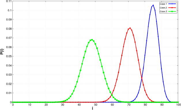
Figure 8.10. Steady-state distributions of gamma distributed interarrival times. For a color version of this figure, see www.iste.co.uk/anisimov/queueing1.zip
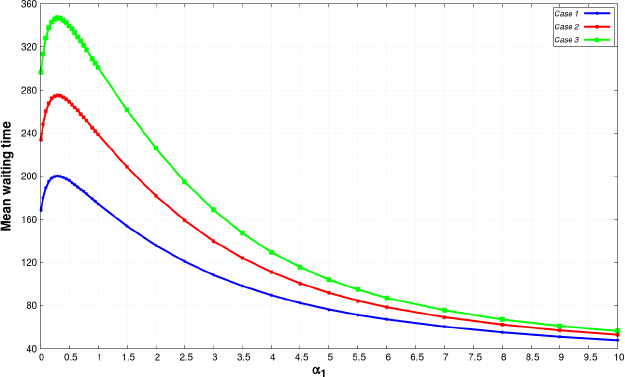
Figure 8.11. Mean waiting time versus shape parameter. For a color version of this figure, see www.iste.co.uk/anisimov/queueing1.zip
In Figures 8.11 and 8.13, the service time distribution of the cases has the following parameters: α = β = 0.5, 1, 2, respectively, and all the other parameters are the same as in Table 8.11. The running parameter is α1 , so in this way the impact of different distributions on the various performance measures can be discovered. First the mean waiting time (Figure 8.11), after an initial jump mean waiting time, starts to monotonically decrease resulting in α1 getting bigger the less time the customers spend in the system. At the end, the values of separate cases are almost equal. As a result (Figure 8.11), it is not surprising how the mean interrupted service time changes as a function of α1 . It is interesting that around α1 ≈ 4.5 we observe that the curves intersect each other.
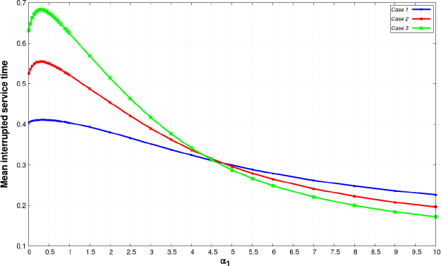
Figure 8.12. Mean interrupted service time versus shape parameter. For a color version of this figure, see www.iste.co.uk/anisimov/queueing1.zip
8.4.4. Gamma distributed retrial times
In this case not just the interarrival but also the retrial time are gamma distributed with the same parameters. Table 8.12 shows the input parameters of this system.
Table 8.12. Numerical values of parameters of gamma distributed retrial times
| Case | N | α | β | γo | γ1 | γ2 | α1 | β1/N |
|---|---|---|---|---|---|---|---|---|
| 1 | 100 | 1 | 1 | 0.1 | 0.1 | 1 | 0.5 | 0.01 |
| 2 | 100 | 1 | 1 | 0.1 | 0.1 | 1 | 1 | 0.01 |
| 3 | 100 | 1 | 1 | 0.1 | 0.1 | 1 | 2 | 0.01 |
Table 8.13 contains the main performance measures in connection with the cases.
Table 8.13. Simulation results
| Case | E(J) | Var(J) | E(T) | Var(T) | E(W) | Var(W) | E(S) | Var(S) | E(IS) |
|---|---|---|---|---|---|---|---|---|---|
| 1 | 81.5384 | 16.9599 | 220.8314 | 82,735.764 | 219.8314 | 82,377.8317 | 0.3398 | 0.1183 | 0.6602 |
| 2 | 70.5912 | 24.3012 | 239.9734 | 105,273.4267 | 238.9734 | 104,918.6389 | 0.4784 | 0.2289 | 0.5217 |
| 3 | 56.6635 | 30.1636 | 261.483 | 146,264.4778 | 260.4827 | 145,919.0907 | 0.626 | 0.3915 | 0.3743 |
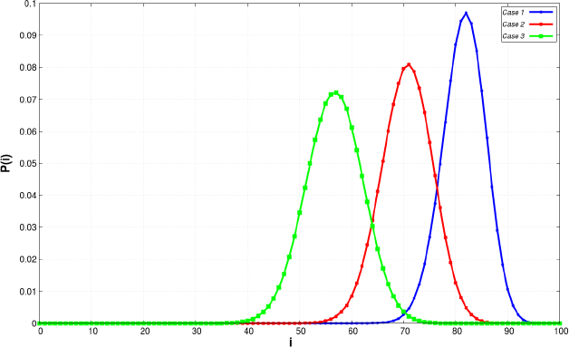
Figure 8.13. Steady-state distributions of gamma distributed retrial times. For a color version of this figure, see www.iste.co.uk/anisimov/queueing1.zip
Let us notice that under this parameter setup this modification has no significant effect on the steady-state distribution (see Figure 8.13). Of course, the mean customers in the system is quite disparate but the distribution remains normal. Also when α1 is less than 1, it results in a higher mean number of customers in the system compared to when it is more than one.
8.4.5. The effect of breakdowns disciplines
In Tóth et al. (2019), the M/G/1//N and G/M/1//N systems were investigated with exponentially distributed operating and repair times. In cases of server failure, two operation modes are considered:
- – the interrupted request gets into the orbit instantaneously (mode 1);
- – the service of the interrupted request is suspended and it continues after repairing the server (mode 2).
8.4.5.1. Scenario A, gamma distributed service time
Table 8.14 shows the input parameters of scenario A.
Table 8.14. Numerical values of model parameters
| Case | N | λ/N | γ0 | γ1 | γ2 | σ / N | α | β |
|---|---|---|---|---|---|---|---|---|
| 1 | 100 | 0.01 | 0.1 | 0.1 | 1 | 0.01 | 0.5 | 0.5 |
| 2 | 100 | 0.01 | 0.1 | 0.1 | 1 | 0.01 | 1 | 1 |
| 3 | 100 | 0.01 | 0.1 | 0.1 | 1 | 0.01 | 2 | 2 |

Figure 8.14. Comparison of steady-state distributions for mode 2. For a color version of this figure, see www.iste.co.uk/anisimov/queueing1.zip
Figure 8.14 shows the steady-state distribution of the investigated cases for operation mode 2. Case 2 is a special case because when parameter α is equal to 1, it results in the exponential distribution. The mean number of customers increases with the increment of parameters α and β and, taking a closer look at the shape of the curves, steady-state distribution of the cases follow normal distribution. Table 8.15 presents the considered performance measures in relation to the different cases.
Figures 8.15–8.17 compare the mean waiting time of the two different operation modes of the investigated cases. Operation mode 1 reflects the mode when the interrupted requests get into the orbit instantaneously, and under operation mode 2, we consider the mode when the service of the interrupted request is suspended and it continues after repairing the server. In all cases, the results confirm the expectation that applying operation mode 2 results in lower mean waiting time. When the values of parameter α and β are higher, the difference between the modes is higher as well. With increasing arrival intensity, we should expect higher waiting times but after λ/N reaches 0.15 it starts to monotonically decrease, which is an interesting phenomenon.
Table 8.15. Numerical results of scenario A
| Case | E(J) | Var(J) | E(T) | Var(T) | E(W) | Var(W) | E(S) | Var(S) |
|---|---|---|---|---|---|---|---|---|
| 1 | 63.0526 | 28.3198 | 170.5618 | 63, 092.8264 | 169.7553 | 62, 855.9266 | 0.3357 | 0.2255 |
| 2 | 69.6114 | 24.6949 | 228.9834 | 97, 974.6274 | 227.8834 | 97, 613.9701 | 0.5022 | 0.2523 |
| 3 | 73.9099 | 21.9244 | 283.1452 | 136, 396.9409 | 281.7728 | 135, 909.2373 | 0.6688 | 0.2238 |
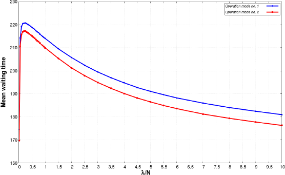
Figure 8.15. Mean waiting time versus intensity of incoming customers of Case 1. For a color version of this figure, see www.iste.co.uk/anisimov/queueing1.zip
Figure 8.15 shows the mean waiting time as a function of failure rate. As it is expected, the mean waiting time increases with the higher failure rate in all cases. Comparing the operation modes, the difference is quite obvious. While using operation mode number 2, the growth seems linear, and in the case of operation mode number 1, the rise is quite significant especially in Case 3.
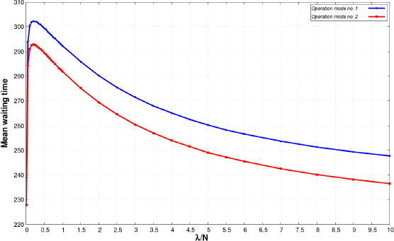
Figure 8.16. Mean waiting time versus intensity of incoming customers of Case 2. For a color version of this figure, see www.iste.co.uk/anisimov/queueing1.zip
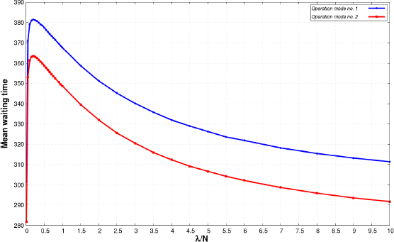
Figure 8.17. Mean waiting time versus intensity of incoming customers of Case 3. For a color version of this figure, see www.iste.co.uk/anisimov/queueing1.zip
8.4.5.2. Scenario B, gamma distributed interarrival time
In scenario B, the distribution of interarrival times of the customers is gamma distributed with parameter λ1 and β1. Table 8.16 presents the numerical values of parameters of scenario B.
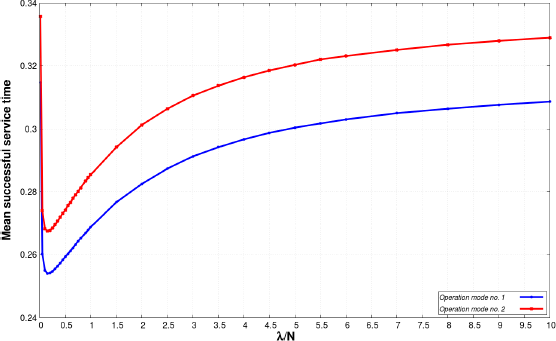
Figure 8.18. Mean successful service time versus intensity of incoming customers of Case 1. For a color version of this figure, see www.iste.co.uk/anisimov/queueing1.zip
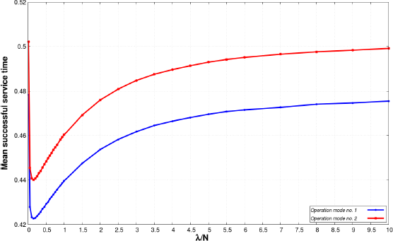
Figure 8.19. Mean successful service time versus intensity of incoming customers of Case 2. For a color version of this figure, see www.iste.co.uk/anisimov/queueing1.zip
Table 8.16. Numerical values of parameters of scenario B
| Case | N | α | β | γo | γ1 | γ2 | σ/N | α1 | β1/N |
|---|---|---|---|---|---|---|---|---|---|
| 1 | 100 | 1 | 1 | 0.1 | 0.1 | 1 | 0.01 | 0.5 | 0.01 |
| 2 | 100 | 1 | 1 | 0.1 | 0.1 | 1 | 0.01 | 1 | 0.01 |
| 3 | 100 | 1 | 1 | 0.1 | 0.1 | 1 | 0.01 | 2 | 0.01 |

Figure 8.20. Mean successful service time versus intensity of incoming customers of Case 3. For a color version of this figure, see www.iste.co.uk/anisimov/queueing1.zip
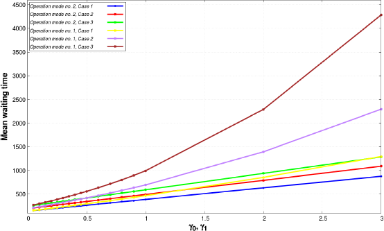
Figure 8.21. Mean waiting time versus intensity of failure rate. For a color version of this figure, see www.iste.co.uk/anisimov/queueing1.zip
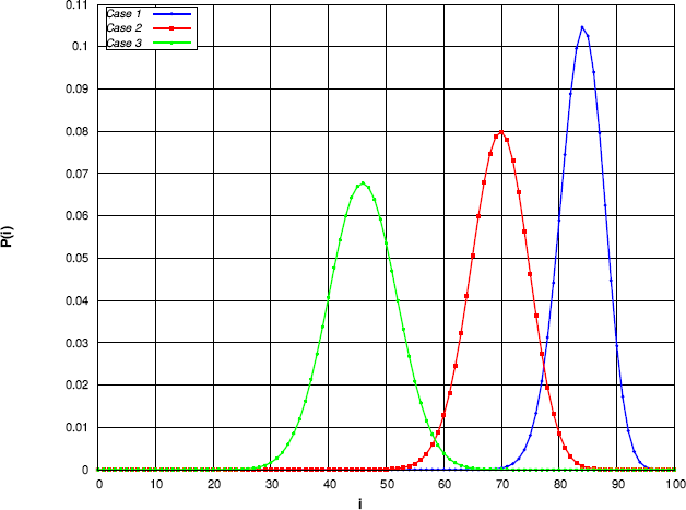
Figure 8.22. Steady-state distributions of scenario B. For a color version of this figure, see www.iste.co.uk/anisimov/queueing1.zip
Table 8.17. Numerical results of scenario B
| Case | E(J) | Var(J) | E(T) | Var(T) | E(W) | Var(W) | E(S) | Var(S) |
|---|---|---|---|---|---|---|---|---|
| 1 | 83.856 | 14.4707 | 259.7716 | 121,328.2493 | 258.6719 | 120,904.8333 | 0.4707 | 0.2232 |
| 2 | 69.5984 | 24.7715 | 228.9076 | 97,997.6219 | 227.8074 | 97,637.2906 | 0.5025 | 0.2525 |
| 3 | 45.9508 | 34.3607 | 170.0134 | 62, 628.4067 | 168.9133 | 62, 379.0441 | 0.5806 | 0.337 |
Figure 8.22 displays the steady-state distributions of Scenario B. Now, the service time is supposed to be exponentially distributed (α = 1). With this modification compared to scenario A, the steady-state distributions still follow a normal distribution and as the value of α1 is increasing, the mean number of requests in the system is decreasing. In Case 3, the mean number of customers in the system is significantly lower among the cases. In Table 8.17, an estimation for the main performance measures can be found in connection with the cases.
The running parameter is α1 and helps to discover the impact of different distributions on the various examined performance measures. Figures 8.23–8.25 show the comparison of the mean waiting time between the two operation modes of the investigated cases. As in scenario A, using operation mode number 2, when the interrupted requests stay at the server in cases of server failure and their services continue after the server is ready to process jobs again, ensures lower mean waiting times. In all cases, the mean waiting time starts to increase till α1 reaches 0.3, then it monotonically decreases. With higher values of α and β , the difference between the operation modes are higher as well.
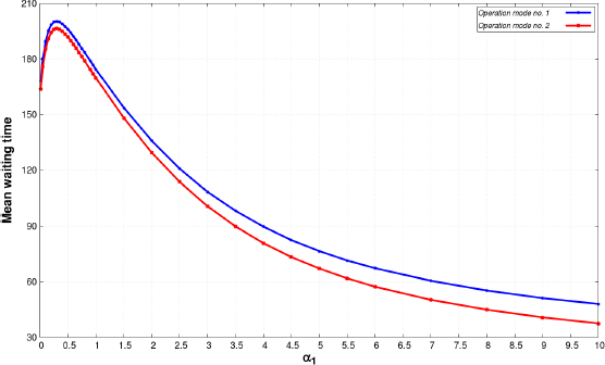
Figure 8.23. Mean waiting time versus shape parameter, α = β =0.5. For a color version of this figure, see www.iste.co.uk/anisimov/queueing1.zip

Figure 8.24. Mean waiting time versus shape parameter, α = β = 1. For a color version of this figure, see www.iste.co.uk/anisimov/queueing1.zip
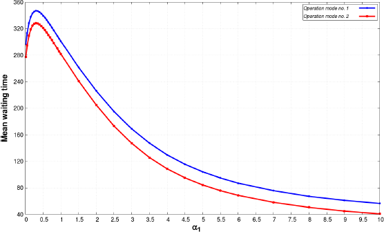
Figure 8.25. Mean waiting time versus shape parameter, α = β =2. For a color version of this figure, see www.iste.co.uk/anisimov/queueing1.zip
Figures 8.26–8.28 show the mean successful service time versus the shape parameter of the interarrival time using both operation mode. As we can see in scenario A, we get what we expected as the usage of operation mode number 2 provides higher values of mean successful service time. The difference is quite high between the applied operation modes in all cases especially when α and β is equal to 0.5. The mean successful service time behaves in reverse compared to the mean waiting time because when the mean waiting time increases the mean successful service time decreases and vice versa.
8.5. Conclusion
In this chapter, tool-supported, numerical, simulation, and asymptotic methods were considered under the condition of an unlimited growing number of sources in a finite-source retrial queue with collisions of customers and an unreliable server. During the survey, several cases and examples were treated and the results of different approaches were compared to each other showing the advantages and disadvantages of the given method. Tables and figures used in this chapter illustrate some special features of these systems. In the near future, the two research groups would like to continue their investigations in this direction including systems with impatient customers, systems embedded in a random environment and systems with two-way communications, just to mention some alternative generalizations.
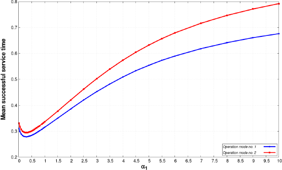
Figure 8.26. Mean successful service time versus shape parameter, α = β = 0.5. For a color version of this figure, see www.iste.co.uk/anisimov/queueing1.zip
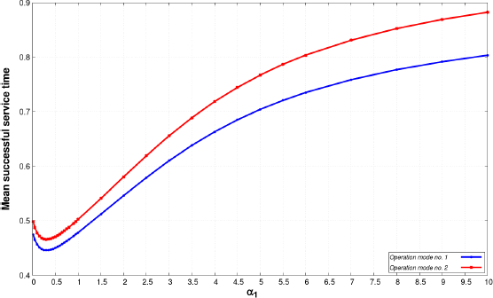
Figure 8.27. Mean successful service time versus shape parameter, α = β = 1. For a color version of this figure, see www.iste.co.uk/anisimov/queueing1.zip
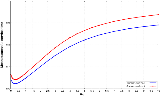
Figure 8.28. Mean successful service time versus shape parameter, α = β = 2. For a color version of this figure, see www.iste.co.uk/anisimov/queueing1.zip
8.6. Acknowledgments
The authors are very grateful to the reviewer for their comments and recommendations, which improved the presentation of the chapter.
The work/publication of J. Sztrik is supported by the EFOP-3.6.1-16-2016-00022 project. The project is co-financed by the European Union and the European Social Fund.
8.7. References
Ali, A.-A., Wei, S. (2015). Modeling of coupled collision and congestion in finite source wireless access systems. Wireless Communications and Networking Conference (WCNC), IEEE, New Orleans, 1113–1118.
Almási, B., Roszik, J., Sztrik, J. (2005). Homogeneous finite-source retrial queues with server subject to breakdowns and repairs. Math. Comput. Model., 42(5–6), 673–682.
Anisimov, V. (1999). Averaging methods for transient regimes in overloading retrial queueing systems. Math. Comput. Model., 30(3–4), 65–78.
Anisimov, V., Sztrik, J. (1989). Asymptotic analysis of some complex renewable systems operating in random environments. European Journal of Operational Research, 41(2), 162–168.
Anisimov, V., Artalejo, J. R. (2001). Analysis of Markov multiserver retrial queues with negative arrivals. Queueing Systems, 39(2-3), 157–182.
Artalejo, J., Corral, A.G. (2008). Retrial Queueing Systems: A Computational Approach. Springer, Berlin.
Bérczes, T., Sztrik, J., Tóth, Á., Nazarov, A. (2017). Performance modeling of finite-source retrial queueing systems with collisions and non-reliable server using MOSEL. International Conference on Distributed Computer and Communication Networks, Springer, Berlin, 248–258.
Bhat, U. N. (2015). An Introduction to Queueing Theory. Modeling and Analysis in Applications. Birkhäuser, Boston.
Bossel, H. (2013). Modeling and Simulation. Springer-Verlag, Berlin.
Cao, Y., Khosla, D., Chen, Y., Huber, D. J. (2018). System and method for real-time collision detection. US Patent 9,934,437.
Choi, B.D., Shin, Y.W., Ahn, W.C. (1992). Retrial queues with collision arising from unslotted CSMA/CD protocol. Queueing Syst., 11(4), 335–356.
Dragieva, V. I. (2014). Number of retrials in a finite source retrial queue with unreliable server. Asia-Pac. J. Oper. Res., 31(2), 23.
Falin, G., Artalejo, J. (1998). A finite source retrial queue. European Journal of Operational Research, 108, 409–424.
Falin, G., Templeton, J.G.C. (1997), Retrial Queues. Chapman and Hall, London.
Fiems, D., Phung-Duc, T. (2017), Light-traffic analysis of random access systems without collisions. Annals of Operations Research, 277(2), 311–327
Gharbi, N., Dutheillet, C. (2011). An algorithmic approach for analysis of finite-source retrial systems with unreliable servers. Computers & Mathematics with Applications, 62(6), 2535–2546.
Gharbi, N., Ioualalen, M. (2006). GSPN analysis of retrial systems with servers breakdowns and repairs. Applied Mathematics and Computation, 174(2), 1151–1168.
Gharbi, N., Mokdad, L., Ben-Othman, J. (2015). A performance study of next generation cellular networks with base stations channels vacations. Global Communications Conference (GLOBECOM), IEEE, 1–6.
Gharbi, N., Nemmouchi, B., Mokdad, L., Ben-Othman, J. (2014). The impact of breakdowns disciplines and repeated attempts on performances of small cell networks. Journal of Computational Science, 5(4), 633–644.
Gómez-Corral, A., Phung-Duc, T. (2016). Retrial queues and related models. Annals of Operations Research, 247(1), 1–2.
Harchol-Balter, M. (2013). Performance Modeling and Design of Computer Systems: Queueing Theory in Action. Cambridge University Press, Cambridge.
Ikhlef, L., Lekadir, O., Aїssani, D. (2016). MRSPN analysis of semi-Markovian finite source retrial queues. Annals of Operations Research, 247(1), 141–167.
Jinsoo, A., Kim, Y., Kwak, J., Son, J. (2018). Wireless communication method for multi-user transmission scheduling, and wireless communication terminal using same. US Patent App. 15/736,968.
Kim, J., Kim, B. (2016). A survey of retrial queueing systems. Annals of Operations Research, 247(1), 3–36.
Kim, J.S. (2010). Retrial queueing system with collision and impatience. Communications of the Korean Mathematical Society, 25(4), 647–653.
Kobayashi, H., Mark, B. L. (2009). System Modeling and Analysis: Foundations of System Performance Evaluation. Pearson Education India, Chennai.
Krishnamoorthy, A., Pramod, P.K., Chakravarthy, S.R. (2014). Queues with interruptions: a survey. TOP, 22(1), 290–320.
Kuki, A., Bérczes, T., Sztrik, J., Kvach, A. (2019). Numerical analysis of retrial queueing systems with conflict of customers. Journal of Mathematical Sciences, 237, 637–683.
Kulkarni, V.G. (2016). Modeling and Analysis of Stochastic Systems. CRC Press, Boca Raton.
Kumar, B.K., Vijayalakshmi, G., Krishnamoorthy, A., Basha, S.S. (2010). A single server feedback retrial queue with collisions. Computers & Operations Research, 37(7), 1247–1255.
Kvach, A. (2014). Numerical research of a Markov closed retrial queueing system without collisions and with the collision of the customers. Proceedings of Tomsk State University. TSU Publishing House, Tomsk, 105–112 (in Russian).
Kvach, A., Nazarov, A. (2015a). Numerical research of a closed retrial queueing system M/GI/1//N with collision of the customers. Proceedings of Tomsk State University. TSU Publishing House, Tomsk, 65–70 (in Russian).
Kvach, A., Nazarov, A. (2015b). Sojourn Time Analysis of Finite Source Markov Retrial Queuing System with Collision. Springer International Publishing, Cham.
Kvach, A., Nazarov, A. (2015c). The research of a closed RQ-system M/GI/1//N with collision of the customers in the condition of an unlimited increasing number of sources. Probability Theory, Random Processes, Mathematical Statistics and Applications, 65–70 (in Russian).
Kwak, B.-J., Rhee, J.-K., Kim, J., Kyounghye, K. (2018). Random access method and terminal supporting the same. US Patent 9,954,754.
Lakaour, L., Aїssani, D., Adel-Aissanou, K., Barkaoui, K. (2018). M/M/1 retrial queue with collisions and transmission errors. Methodology and Computing in Applied Probability, 1–12.
Lakatos, L., Szeidl, L., Telek, M. (2013). Introduction to Queueing Systems with Telecommunication Applications. Springer, New York.
Law, A.M., Kelton, W.D. (1991). Simulation Modeling and Analysis. McGraw-Hill, New York.
Nazarov, A., Kvach, A., Yampolsky, V. (2014). Asymptotic Analysis of Closed Markov Retrial Queuing System with Collision. Springer International Publishing, Cham.
Nazarov, A., Moiseeva, S.P. (2006). Methods of Asymptotic Analysis in Queueing Theory. NTL Publishing House of Tomsk University, Tomsk (in Russian).
Nazarov, A., Sudyko, E. (2010). Method of asymptotic semi-invariants for studying a mathematical model of a random access network. Probl. Inf. Transm., 46(1), 86–102.
Nazarov, A., Sztrik, J., Kvach, A. (2017a). Comparative analysis of methods of residual and elapsed service time in the study of the closed retrial queuing system M/GI/1//N with collision of the customers and unreliable server. International Conference on Information Technologies and Mathematical Modelling, 97–110.
Nazarov, A., Sztrik, J., Kvach, A. (2017b). Some features of a finite-source M/GI/1 retrial queuing system with collisions of customers. International Conference on Distributed Computer and Communication Networks, 186–200.
Nazarov, A., Sztrik, J., Kvach, A. (2017c). Some features of a finite-source M/GI/1 retrial queuing system with collisions of customers. International Conference on Distributed Computer and Communication Networks, 79–86.
Nazarov, A., Sztrik, J., Kvach, A. (2018). A survey of recent results in finite-source retrial queues with collisions. In Information Technologies and Mathematical Modelling. Queueing Theory and Applications, Dudin, A., Nazarov, A., Moiseev, A. (eds). Springer, Berlin.
Nazarov, A., Sztrik, J., Kvach, A., Bérczes, T. (2018). Asymptotic analysis of finite-source M/M/1 retrial queueing system with collisions and server subject to breakdowns and repairs. Annals of Operations Research, 277(2), 213–229.
Nazarov, A., Sztrik, J., Kvach, A., Tóth, A. (2018). Asymptotic sojourn time analysis of Markov finite-source M/M/1 retrial queueing system with collisions and server subject to breakdowns and repairs. Probability in the Engineering and Informational Sciences, 33(3), 387–403.
Nazarov, A., Terpugov, A. (2004). Theory of Mass Service. NTL Publishing House of Tomsk University, Tomsk (in Russian).
Peng, Y., Liu, Z., Wu, J. (2014). An M/G/1 retrial G-queue with preemptive resume priority and collisions subject to the server breakdowns and delayed repairs. J. Appl. Math. Comput., 44(1–2), 187–213.
Reith III, H. C. (2017). System and method for collision detection and avoidance for network communications. US Patent 9,553,828.
Roszik, J. (2004). Homogeneous finite-source retrial queues with server and sources subject to breakdowns and repairs. Ann. Univ. Sci. Budap. Rolando Eotvos, Sect. Comput., 23, 213–227.
Rubinstein, R. Y., Kroese, D. P. (2016). Simulation and the Monte Carlo Method. John Wiley & Sons, Hoboken.
Stewart, W. J. (2009). Probability, Markov Chains, Queues, and Simulation: The Mathematical Basis of Performance Modeling. Princeton University Press, Princeton.
Sztrik, J. (2005). Tool supported performance modelling of finite-source retrial queues with breakdowns. Publicationes Mathematicae, 66, 197–211.
Sztrik, J., Almási, B., Roszik, J. (2006). Heterogeneous finite-source retrial queues with server subject to breakdowns and repairs. Journal of Mathematical Sciences, 132, 677–685.
Takeda, T., Yoshihiro, T. (2017). A distributed scheduling through queue-length exchange in CSMA-based wireless mesh networks. Journal of Information Processing, 25, 174–181.
Tóth, Á., Bérczes, T., Sztrik, J., Kuki, A. (2019). Comparison of two operation modes of finite-source retrial queueing systems with collisions and non-reliable server by using simulation. Journal of Mathematical Sciences, 237, 846–857.
Tóth, Á., Bérczes, T., Sztrik, J., Kvach, A. (2017). Simulation of finite-source retrial queueing systems with collisions and a non-reliable server. International Conference on Distributed Computer and Communication Networks, 146–158. Springer.
Wang, J., Zhao, L., Zhang, F. (2010). Performance analysis of the finite source retrial queue with server breakdowns and repairs. Proceedings of the 5th International Conference on Queueing Theory and Network Applications, ACM, 169–176.
Wang, J., Zhao, L., Zhang, F. (2011). Analysis of the finite source retrial queues with server breakdowns and repairs. Journal of Industrial and Management Optimization, 7(3), 655–676.
Wentink, M. (2017). Collision avoidance systems and methods. US Patent App. 15/401,606.
Wüchner, P., Sztrik, J., de Meer, H. (2010). Finite-source retrial queues with applications. Proceedings of 8th International Conference on Applied Informatics, Eger, Hungary, 275–285.
Yao, J. (2016). Asymptotic Analysis of Service Systems with Congestion-Sensitive Customers. Columbia University, New York City.
Yeo, G. M., Kim, Y. I., Park, D. G., Song, S. Y., Lee, Y. T., Lee, H. W. (2017). Control method and apparatus for collision avoidance in low-power wireless sensor communication. US Patent App. 15/361,194.
Zhang, F., Wang, J. (2013). Performance analysis of the retrial queues with finite number of sources and service interruptions. Journal of the Korean Statistical Society, 42(1), 117–131.