
10
Time-varying Queues: a Two-time-scale Approach
George YIN1, Hanqin ZHANG2 and Qing ZHANG3
1Wayne State University, Detroit, USA
2School of Business, National University of Singapore, Singapore
3University of Georgia, Athens, USA
This chapter is concerned with time-varying queues with customer abandonment and finite waiting rooms. A two-time-scale Markov chain approach is adopted to study the performance measures of the system including the queue length, the probabilities of customer reneging and the abandonment for such time-varying queues. Both moderate deviations and large deviations are considered when time scale separation is in effect. In the study of large deviations, the calculation of rate function is crucial. In this chapter, general expression of the rate function is provided. At the same time, a numerical example is also included to illustrate a related rate function calculation.
10.1. Introduction
Many queueing systems, that arise in applications are time varying in nature. These queueing systems include service systems such as customer contact centers, patient flows in emergency departments and ward management in hospitals. In these systems, either customer arrival rates, service rates or hazard rates of customer abandonment are time dependent. There are several empirical studies that have been conducted on such time inhomogeneity (see, for instance, Armony et al. (2015); Batt and Terwiesch (2015); Yom-Tov and Mandelbaum (2014), among others).
By and large, there are a few ways to treat these time-varying queues. One way is to apply time-invariant (or time-homogeneous or stationary) queues to approximate the time-inhomogeneous queues. When building the models for the time-stationary queues, usually we can establish three different stationary models based on the various managerial motivation. One of the models is to assume that the customer arrival rate and service rate are time dependent but change sufficiently slowly. Thus, the system performance measures such as queue length and waiting time at running time t can be approximated by that of the steady-state performance measures of the time stationary queue with the customer arrival rate and service rate being fixed at time t. This approximation is called a pointwise-stationary approximation in the queueing literature (see Green and Kolesar (1991); Whitt (1991)). Another two time-stationary models are constructed by considering the quality of service at all times. For example, to analyze the time-varying queue over time interval [0, T], we use either the maximum of the customer arrival rates over [0, T] or the average of the customer arrival rates over [0, T] instead of time-varying customer arrival rates to construct the time-stationary queue, as it is referred to in queueing literature. Apart from applying time-stationary queues, another way to study the time-varying queues is to use the many-server queue idea. In this setting, the customer arrival rate and the number of servers are assumed to be large. Then the system performance measures can be approximated by a Gaussian process or a function of a Gaussian process (see Liu (2018); Liu and Whitt (2014)). A survey on the vast literature on time-varying queues has been provided by Whitt (2018).
In contrast with traditional approaches, we develop a two-time-scale Markov chain approach to analyze the time-varying queues in this chapter. Treating time-inhomogeneous Markov chains with two-time scales, Yin and Zhang (2013) developed the approximation schemes based on time-scale separation. The central theme is the use of the so-called quasi-stationary (or quasi-steady state) distributions (see Chapter 2 of Yin and Zhang (2013) for a definition). A quasi-steady-state distribution is roughly like a steady-state distribution. However, the distribution can be time dependent. The time dependence arises from the two-time-scale formulation, in which one has two time scales. One of them is real running time t, and the other is a “stretched time” t/ε. Holding t as a “constant” and letting ε → 0 yields a limit, which is t dependent. For further details, we refer the reader to Yin and Zhang (2013) (see also Yin et al. (2013) and references therein). Such an approximation result is rather convenient for us to carry out the study in the time-varying queues. Here, we use the phrase “quasi” to reflect the time dependence involved. We model the queue length process as a continuous-time Markov chain. When the customer arrival rate and the number of servers get larger and larger, the two-time-scale feature in the Markov chain emerges. Using a small parameter ε > 0 to highlight the time scale separation, the aforementioned feature is pronounced when ε is sufficiently small. One of the central issues in the approximation of the time-varying queues with two-time scales is to closely characterize the approximation by looking at the deviation of the original occupation measures from that of the quasi-steady-state measures. A closed caption of this property can be done by using large deviations analysis. A related work on diffusion approximation can be found in the work of Anisimov (1995).
Because of the time-scale separation, within a short period of time, the queueing system will reach its quasi-steady state. One important question concerns the probability of the rates of convergence to the quasi-steady distribution. The answer to such a question is beyond the usual normal deviations range of the errors. A pertinent analysis is based on larger than normal deviations. In this chapter, we use the large deviations principal for two-time-scale non-homogeneous Markov chains to analyze the queue length process and associated probabilities, which characterizes the quality of service and the efficiency of the systems. In addition, in this chapter, we also characterize the quality of approximation by examining deviations that are larger than the usual normal deviations but are not quite in the large deviation range. This is the study of moderate deviations.
The rest of the chapter is organized as follows. In section 10.2, we give a mathematical description for our time-varying queues. Section 10.3 demonstrates how to use the large deviation principal to analyze the time-varying queues. The chapter concludes in section 10.4 with some further remarks.
10.2. Time-varying queues
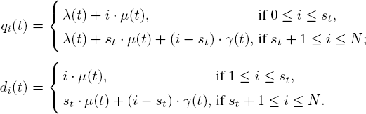
We consider the Mt/Mt/st + Mt/N model, in which the customer arrival process is a non-stationary Poisson process with rate λ(t); the system has st identical servers, and their service rate is μ(t) at time t. The arriving customers are impatient and their patient times are independent and follow exponential distribution with parameter γ(t) at time t. Here, N is the system capacity, that is, the system is a loss system and arriving customers will be forced to balk when the system reaches its capacity, that is, when there are N customers in the system. Let Q(t) represent the number of customers in the system at time t. By the memoryless property of the customer arrival process, service time and patience time, we know that {Q(t) : t ≥ 0} is a Markov process with the state space {0, 1,..., N}. At time t, the system service completion rate is
and the customer abandonment rate is
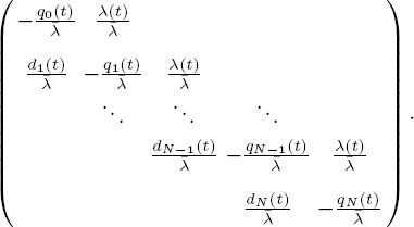
Based on the above observation, we know that the generator ![]() of the queue length process {Q(t) : t ≥ 0} is given by
of the queue length process {Q(t) : t ≥ 0} is given by
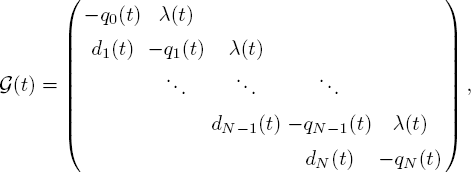
where
The above formulation regarding the number of servers at time t in the system is very general and can capture many interesting features from practical considerations. Under such a setup, we can consider the following special situations.
PROBLEM 10.1.– First, we consider a dynamic staffing problem. In particular, there are k thresholds related to the number of customers in the system to dynamically adjust the staffing levels. Namely, for given k thresholds
and k staffing levels
when the number of customers in the system at time t is strictly larger than nl but less than or equal to nl+1 with 1 = 0, . . . ,k − 1, we use sl+1 servers to handle the customer service. With this staffing policy, we have that
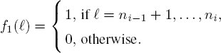
and for i = nl + 1, . . . , nl + 1 with 0 ≤ l ≤ k − 1,
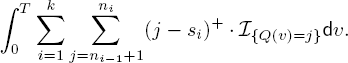
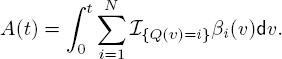
To evaluate the efficiency of the staffing policy for this problem, we need to analyze the probability distribution for t ≥ 0,


![]() indicates the cumulative time that the system uses si servers to handle customer service during time interval [0, t].
indicates the cumulative time that the system uses si servers to handle customer service during time interval [0, t].
PROBLEM 10.2.– Next, consider a time-dependent staffing policy. Formally, the time interval [0, ∞) is divided into a few subintervals,
and the staffing level at interval [tl,tl+1) is given by s = sl+1 for l = 0, . . . ,k − 1. Thus, for t ∈ [tl,tl) with l = 1, . . . ,k,
Similarly, to analyze the customer loss probability, we introduce
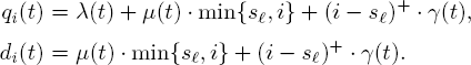
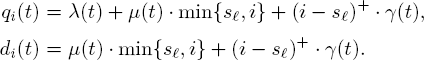
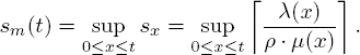
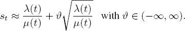
PROBLEM 10.3.– Finally, we consider the staffing problem based on the ratio of the customer arrival rate to service rate. At time t, the staffing level st is chosen such that ![]() holds with the smallest positive integer st. Here, ρ is determined in advance; usually it shows us the system service quality. Thus, for any time t, with the customer arrival rate λ(t) and each individual server’s service rate μ(t), we have
holds with the smallest positive integer st. Here, ρ is determined in advance; usually it shows us the system service quality. Thus, for any time t, with the customer arrival rate λ(t) and each individual server’s service rate μ(t), we have

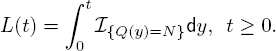
Let
We consider the probability distribution

This shows the cumulative time that the system takes to handle the customer service during time interval [0, t] using the maximum number of servers.
With the setting of the three problems given above, in what follows, we develop a two-time-scale approach to analyze the probability distributions of ![]() and L(t). A crucial point is to let the generator of the queue length process depend on a small parameter. As the small parameter goes to 0, the system may be replaced by an average one.
and L(t). A crucial point is to let the generator of the queue length process depend on a small parameter. As the small parameter goes to 0, the system may be replaced by an average one.
10.3. Main results
We divide this section into several subsections. We first consider large deviations of the two-time-scale queues and then provide some discussion on a relevant computational method. This is followed by applications in various queues. Additional considerations on moderate deviations will also be discussed.
10.3.1. Large deviations of two-time-scale queues
Consider a general finite-state continuous-time Markov chain {Xε (t) : t ≥ 0} depending on a small parameter ε > 0 with a generator ![]() such that
such that
where ![]() is given by [10.1], is irreducible and is twice continuously differentiable with respect to t. Note that although [10.6] only has a fast varying part, the system is still a two-time scale queue. As alluded to previously, there is natural time t and also stretched time t/ε. Let S = {0, 1, . . . ,N} denote its state space, and
is given by [10.1], is irreducible and is twice continuously differentiable with respect to t. Note that although [10.6] only has a fast varying part, the system is still a two-time scale queue. As alluded to previously, there is natural time t and also stretched time t/ε. Let S = {0, 1, . . . ,N} denote its state space, and
For a fixed T > 0, consider a k-dimensional random variable

Then using the occupation measure, it is readily seen that
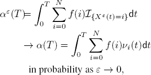
where ν(t) = (ν0(t), . . . ,νN(t)) is the quasi-stationary distribution. Note that the random variable αε(T) defined above is used to capture the performance measures in problems 10.1–10.3.
For example, consider problem 10.1. Let k = 1 in [10.8] and
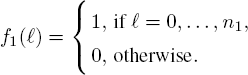
Then we have [10.2] with t = T in problem 10.1. That is,
In general, consider ![]() for i = 2, . . . ,k. Let k = 1 and
for i = 2, . . . ,k. Let k = 1 and
Then we have [10.3] with t = T in problem 10.1. That is,
Consider problem 10.2. Let k = 1 in [10.8] and
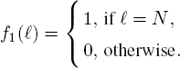
We have that Lε (T) = αε (T) in [10.4].
Similarly for problem 10.3, let
with

Furthermore, let k = N + 1 in [10.8] and for l ∈ S,
Then Mε (T) = αε (T) in [10.5]. Here, we note that f (∙) given by [10.7] has been modified to be dependent on t.
Now we give a systematic way to estimate the probability distribution of random variable αε(T) given in [10.8]. From theorem 4.2 in He et al. (2011), we have the following result.
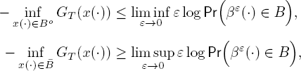
THEOREM 10.1.– For any B ⊆ ℝk, let Bo and ![]() be the interior and closure of B in ℝk, respectively. Then
be the interior and closure of B in ℝk, respectively. Then

where
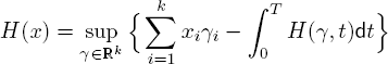
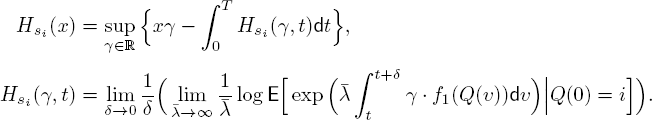
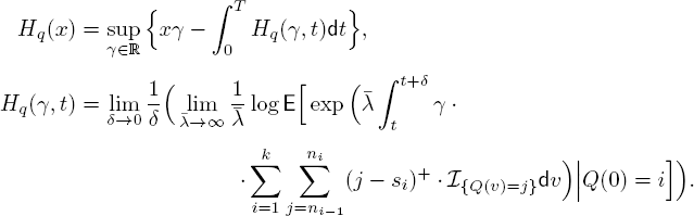
with for y ∈ ℝk and t ≥ 0,

According to theorem 10.1, to get the probabilistic estimate of αε (T) in [10.8], we need to find the function H (∙). Although the analytic form of H(∙) is available and given above, the calculation in general is not straightforward. Nevertheless, in what follows, we demonstrate how to compute H (∙) in certain cases.
10.3.2. Computation of H (y, t)
In this section, we consider a special case of ![]() and demonstrate how to compute H(y, t). We consider {Xε (t) : t ≥ 0} as a birth–death process with the state space S and the generator
and demonstrate how to compute H(y, t). We consider {Xε (t) : t ≥ 0} as a birth–death process with the state space S and the generator ![]() /ε with
/ε with ![]() given by [10.1].
given by [10.1].
For i = 0, 1, . . . , N, let
where ![]() is given in [10.7].
is given in [10.7].
If ![]() is a piecewise constant matrix, then we can assume it is right continuous with left-hand limit. Otherwise, we can modify it by taking its left-hand limit and use
is a piecewise constant matrix, then we can assume it is right continuous with left-hand limit. Otherwise, we can modify it by taking its left-hand limit and use ![]() instead
instead
In order to evaluate the function H(y, t), we only have to examine the case with constant ![]() We focus on constant
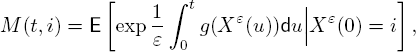
We focus on constant ![]() in this section. Let M (t) = (M (t, 0),M (t, 1), . . . , M (t,N ))’ and let A = diagg(0), g(1), . . . , g(N) +
in this section. Let M (t) = (M (t, 0),M (t, 1), . . . , M (t,N ))’ and let A = diagg(0), g(1), . . . , g(N) + ![]() . Then, the Feynman–Kac formula yields the differential equation
. Then, the Feynman–Kac formula yields the differential equation
Its solution is given by
EXAMPLE 10.1.– To illustrate a possible way to compute H(y,t), we specialize further and consider a 3 × 3 constant matrix ![]() in which the matrix A admits three distinct real eigenvalues η0 > η1 > η2. Then there exists an invertible matrix S such that
in which the matrix A admits three distinct real eigenvalues η0 > η1 > η2. Then there exists an invertible matrix S such that
It follows that
Then we can write it as

for some constants cij. For each i = 0, 1, 2, let j0(i) = min{j : cij ≠ 0}. Then it is easy to see
Note that H (y, t) depends only on y when ![]() is a constant matrix. When
is a constant matrix. When ![]() changes with t, so does H (y,t).
changes with t, so does H (y,t).
In particular, we let
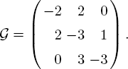
Then, the matrix satisfies the eigenvalue condition. The limit H (y,t) is given in Figure 10.1.
To proceed, we come back to the three problems discussed briefly in the last section.
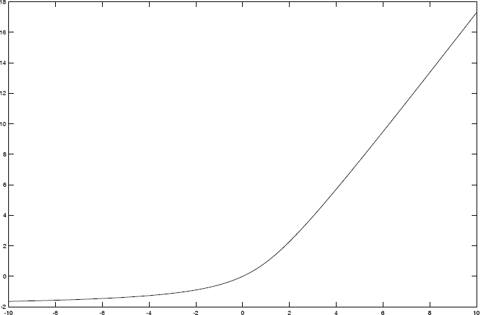
Figure 10.1. Function H(y) = H(y,t)
10.3.3. Applications to queueing systems
In many-server queues, the customer arrival rate is usually assumed to be very high, and the staffing level is also high regardless of which regime it takes among efficiency-driven, quality-driven, and both quality- and efficiency-driven regimes. Consider Mt/Mt/st + Mt/N given by [10.1]. At time t, if the system is under the efficiency-driven regime, we have
while under the quality-driven regime,
and under the quality- and efficiency-driven regime,
For a given time interval [0, T], let
Under the setting of many-server queues, we assume that
This assumption makes us consider ![]() to be ε in theorem 10.1. The generator given by [10.1] can then be written as
to be ε in theorem 10.1. The generator given by [10.1] can then be written as

Now we look at the cumulative time over [0, T] in which the arriving customers get balking for problems 10.1–10.3. From [10.4], this is given by L(T). In view of [10.13] and theorem 10.1, we have that for any ![]() and large enough
and large enough ![]()
where

Now for problem 10.1, we have that for any ![]() and large enough
and large enough ![]() ,
,
where
Here, f1(∙) is defined in [10.9] and [10.11] for i = 1 and i = 2, . . . ,k, respectively. Now consider its queue length given by
For any ![]() and large enough
and large enough ![]() ,
,

where
Note that equations [10.20]–[10.21] and [10.23] are concerned with a fixed time T. Now we look at the situation in which T is not fixed but time varying. In view of [10.8], consider the k-dimensional process {βε(t) : t ≥ 0} given by

where f (∙) is defined by [10.7].
For T > 0, let Ck [0, T] denote the set of all the continuous functions g( ∙): [0, T] → ℝk, and ![]() and h(0) = x}. From theorem 5.1 in He et al. (2011), we have the following:
and h(0) = x}. From theorem 5.1 in He et al. (2011), we have the following:
THEOREM 10.2.– For each ![]() ,
,
where Bo and ![]() are the interior and closure of B in
are the interior and closure of B in ![]() with the uniform metric, and
with the uniform metric, and

with y ∈ ℝk and t ≥ 0,

where H (y,t) is defined in theorem 10.1.
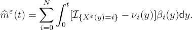
Consider the process generated by the cumulative time during which the arriving customers get balking for problems 10.1–10.3. Consider L(t) given by [10.4]. In more detail, the process {L(t) : t ≥ 0} characterizes the periods over [0, ∞) that indicate when the customer reneging occurs. Then theorem 10.2 shows that for any subset B of ![]() and large enough
and large enough ![]()
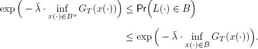
Going along the same line of [10.24], by [10.21] and [10.23], we can give the upper and lower bounds for

Finally, we look at Mε(T) given in [10.5]. To this end, in view of [10.15], we consider the general Markov chain {Xε(t) : t ≥ 0} given by [10.6].
Here, β(t) so that β(t) = (β1(t), . . . , βk(t))’ ∈ ℝk is a step function on [0, T], and
is the quasi-steady-state distribution of the queue with the corresponding ![]() (y) in [10.6]. From theorems 3.1 and 3.2 of He and Yin (2014), we have the following result of moderate deviations. The moderate deviations are reflected from the choice of the parameter κ ∈ (0, 0.5). The moderate deviations together with the large deviations give us a complete characterization of the approximating errors. In what follows, we first state a result for
(y) in [10.6]. From theorems 3.1 and 3.2 of He and Yin (2014), we have the following result of moderate deviations. The moderate deviations are reflected from the choice of the parameter κ ∈ (0, 0.5). The moderate deviations together with the large deviations give us a complete characterization of the approximating errors. In what follows, we first state a result for ![]() .
.
THEOREM 10.3.– There exists a functional ![]() such that
such that

Moreover, for each l = 1, . . . ,k and κ ∈ (0, 0.5),

where C(t) is the Hessian matrix of ![]() (y, t) at y = 0, i.e.
(y, t) at y = 0, i.e.

Let (![]() ) be the quasi-steady-state distribution of the queue length with the generator
) be the quasi-steady-state distribution of the queue length with the generator
Now we give the probability estimate for Mε(T) given in [10.5]. Define
where I(t) is defined in [10.14]. Then it follows from [10.15] that

From theorem 10.3, there exists a functional ![]() such that
such that

Consider the cumulative time in which the customer abandonment can occur for problem 10.2. That is,

Recall that the problem is related to the time-dependent staffing. Formally, the staffing level at interval [tl,tl+1) is given by s = sl+1 with
Now define β(t) = (β1(t), . . . , βN(t)) by
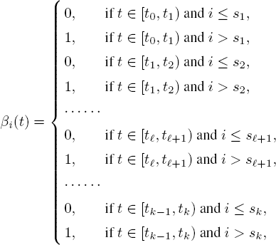
i = 1, . . . , N. Then we have
Similar to the discussion for problem 10.3 (see [10.28]), we have that there exists a functional ![]() (∙, ∙) : ℝk × [0, ∞] → ℝ such that
(∙, ∙) : ℝk × [0, ∞] → ℝ such that
10.4. Concluding remarks
Time-varying queues are much more difficult to handle compared to the time-invariant systems. To face the challenges, we used the large deviations principle developed for the two-time-scale Markov chains to analyze the probabilities for some performance measures in time-varying queues. We also provided moderate deviations analysis for the queueing systems. These performance measures include the abandonment process, the customer balking probability and facility use. The significance of the large deviations and moderate deviations results indicates that tail probabilities of interest are exponentially small, which gives us tight error bounds. It is clear that the quantity of crucial importance is the rate function. Noting [10.20]–[10.21], [10.23]–[10.24], [10.28] and [10.30], however, we only give theoretically the upper and lower bounds or approximation for these probabilities. It is challenging to find the exact analytic or closed-form expressions for the functions such as ![]() for the general generator given by [10.19]. Hence, it is also rather difficult to find the precise expression of the rate function. In our future work, we will develop numerical methods to systematically and numerically compute these values and the rate functions. From another perspective, Koroliuk and Limnios (2001) considered semi-Markov processes and various applications. It will be a worthwhile effort to see how the approach we presented in this chapter can be applied to semi-Markov processes and applications in queueing systems with the renewal arrival or the general service time (see Çinlar 1975). In Anisimov (1992, 2002, 2008), Anisimov studied averaging principles for switching processes. In particular, an idea of quasi-ergodicity was brought in. It seems that this idea may have some connections to the quasi-steady-state distribution used in our approach. To further look into this and study properties, such a large deviation is another direction of worthwhile effort.
for the general generator given by [10.19]. Hence, it is also rather difficult to find the precise expression of the rate function. In our future work, we will develop numerical methods to systematically and numerically compute these values and the rate functions. From another perspective, Koroliuk and Limnios (2001) considered semi-Markov processes and various applications. It will be a worthwhile effort to see how the approach we presented in this chapter can be applied to semi-Markov processes and applications in queueing systems with the renewal arrival or the general service time (see Çinlar 1975). In Anisimov (1992, 2002, 2008), Anisimov studied averaging principles for switching processes. In particular, an idea of quasi-ergodicity was brought in. It seems that this idea may have some connections to the quasi-steady-state distribution used in our approach. To further look into this and study properties, such a large deviation is another direction of worthwhile effort.
10.5. References
Anisimov, V. (1992). Averaging principle for switching processes. Theory Probab. Math. Statist., 46, 1–10.
Anisimov, V. (1995). Switching processes: Averaging principle, diffusion approximation and applications. Acta Appl. Math., 40, 95–141.
Anisimov, V. (2002). Diffusion approximation in overloaded switching queueing models. Queueing Syst., 40, 141–180.
Anisimov, V. (2008). Switching Processes in Queueing Models. ISTE Ltd, London, and Wiley, New York.
Armony, M., Israelit, S., Mandelbaum, A., Marmor, Y.N., Tseytlin, Y., Yom-Tov, G. (2015). On patient flow in hospitals: A data-based queueing-science perspective. Stochastic Syst., 5, 146–194.
Batt, R.J., Terwiesch, C. (2015). Waiting patiently: An empirical study of queue abandonment in an emergency department. Management Sci., 61, 39–59.
Çinlar, E., (1975). Introduction to Stochastic Processes. Prentice-Hall, Englewood Cliffs.
Green, L.V., Kolesar, P.J. (1991). The pointwise stationary approximation for queues with nonstationary arrivals. Management Sci., 37, 84–97.
He, Q., Yin, G. (2014). Moderate deviations for time-varying dynamic systems driven by non-homogeneous Markov chains with two-time scales. Stochastics, 86, 527–550.
He, Q., Yin, G., Zhang, Q. (2011). Large deviations for two-time scale systems driven by non-homogeneous Markov chains and associated optimal control problems. SIAM J. Control Optim., 49, 1737–1765.
Koroliuk, V.S., Limnios, N. (2005). Stochastic Systems in Merging Phase Space. World Scientific Publishing Co. Pte. Ltd., Hackensack.
Liu, Y. (2018). Staffing to stabilize the tail probability of delay in service systems with time-varying demand. Oper. Res., 66, 514–534.
Liu, Y., Whitt, W. (2014). Many-server heavy-traffic limit for queues with time-varying parameters. Ann. Appl. Probab., 24, 378–421.
Whitt, W. (1991). The pointwise stationary approximation for Mt/Mt/s queues is asymptotically correct as the rates increase. Management Sci., 37, 307–314.
Whitt, W. (2018). Time-varying queues. Queueing Models Service Management, 1, 79–164.
Yin, G., Zhang, Q. (2013). Continuous-Time Markov Chains and Applications: A Two-Time-Scale Approach, 2nd edition. Springer, New York.
Yin, G., Zhang, H.Q., Zhang, Q. (2013). Applications of Two-Time-Scale Markovian Systems. Science Press, Beijing.
Yom-Tov, G., Mandelbaum, A. (2014). Erlang-R: A time-varying queue with reentrant customers, in support of healthcare staffing. Manufacturing Service Oper. Management, 16, 283–299.
This research was supported in part by the Army Research Office under grant W911NF-19-1-0176, the Social Science Research Council (Singapore), MOE2016-SSRTG-059 and the Simons Foundation under 235179.