
Behavior of a Sender
Media Capture and Compression
Generating RTP Packets
Behavior of a Receiver
Packet Reception
The Playout Buffer
Adapting the Playout Point
Decoding, Mixing, and Playout
In this chapter we move on from our discussion of networks and protocols, and talk instead about the design of systems that use RTP. An RTP implementation has multiple aspects, some of which are required for all applications; others are optional depending on the needs of the application. This chapter discusses the most fundamental features necessary for media capture, playout, and timing recovery; later chapters describe ways in which reception quality can be improved or overheads reduced.
We start with a discussion of the behavior of a sender: media capture and compression, generation of RTP packets, and the under-lying media timing model. Then the discussion focuses on the receiver, and the problems of media playout and timing recovery in the face of uncertain delivery conditions. Key to receiver design is the operation of the playout buffer, and much of this chapter is spent on this subject.
As noted in Chapter 1, An Introduction to RTP, a sender is responsible for capturing audiovisual data, whether live or from a file, compressing it for transmission, and generating RTP packets. It may also participate in error correction and congestion control by adapting the transmitted media stream in response to receiver feedback. Figure 1.2 in Chapter 1 shows the process.
The sender starts by reading uncompressed media data—audio samples or video frames—into a buffer from which encoded frames are produced. Frames may be encoded in several ways depending on the compression algorithm used, and encoded frames may depend on both earlier and later data. The next section, Media Capture and Compression, describes this process.
Compressed frames are assigned a timestamp and a sequence number, and loaded into RTP packets ready for transmission. If a frame is too large to fit into a single packet, it may be fragmented into several packets for transmission. If a frame is small, several frames may be bundled into a single RTP packet. The section titled Generating RTP Packets later in this chapter describes these functions, both of which are possible only if supported by the payload format. Depending on the error correction scheme in use, a channel coder may be used to generate error correction packets or to reorder frames for interleaving before transmission (Chapters 8 and 9 discuss error concealment and error correction). The sender will generate periodic status reports, in the form of RTCP packets, for the media streams it is generating. It will also receive reception quality feedback from other participants, and it may use that information to adapt its transmission. RTCP was described in Chapter 5, RTP Control Protocol.
The media capture process is essentially the same whether audio or video is being transmitted: An uncompressed frame is captured, if necessary it is transformed into a suitable format for compression, and then the encoder is invoked to produce a compressed frame. The compressed frame is then passed to the packetization routine, and one or more RTP packets are generated. Factors specific to audio/video capture are discussed in the next two sections, followed by a description of issues raised by prerecorded content.
Considering the specifics of audio capture, Figure 6.1 shows the sampling process on a general-purpose workstation, with sound being captured, digitized, and stored into an audio input buffer. This input buffer is commonly made available to the application after a fixed number of samples have been collected. Most audio capture APIs return data from the input buffer in fixed-duration frames, blocking until sufficient samples have been collected to form a complete frame. This imposes some delay because the first sample in a frame is not made available until the last sample has been collected. If given a choice, applications intended for interactive use should select the buffer size closest to that of the codec frame duration, commonly either 20 milliseconds or 30 milliseconds, to reduce the delay.

Uncompressed audio frames can be returned from the capture device with a range of sample types and at one of several sampling rates. Common audio capture devices can return samples with 8-, 16-, or 24-bit resolution, using linear, µ-law or A-law quantization, at rates between 8,000 and 96,000 samples per second, and in mono or stereo. Depending on the capabilities of the capture device and on the media codec, it may be necessary to convert the media to an alternative format before the media can be used—for example, changing the sample rate or converting from linear to µ-law quantization. Algorithms for audio format conversion are outside the scope of this book, but standard signal-processing texts give a range of possibilities.
Captured audio frames are passed to the encoder for compression. Depending on the codec, state may be maintained between frames—the compression context—that must be made available to the encoder along with each new frame of data. Some codecs, particularly music codecs, base their compression on a series of uncompressed frames and not on uncompressed frames in isolation. In these cases the encoder may need to be passed several frames of audio, or it may buffer frames internally and produce output only after receiving several frames. Some codecs produce fixed-size frames as their output; others produce variable-size frames. Those with variable-size frames commonly select from a fixed set of output rates according to the desired quality or signal content; very few are truly variable-rate.
Many speech codecs perform voice activity detection with silence suppression, detecting and suppressing frames that contain only silence or background noise. Suppressed frames either are not transmitted or are replaced with occasional low-rate comfort noise packets. The result can be a significant savings in network capacity, especially if statistical multiplexing is used to make effective use of limited-capacity channels.
Video capture devices typically operate on complete frames of video, rather than returning individual scan lines or fields of an interlaced image. Many offer the ability to subsample and capture the frame at reduced resolution or to return a subset of the frames. Frames may have a range of sizes, and capture devices may return frames in a variety of formats, color spaces, depths, and subsampling.
Depending on the codec used, it may be necessary to convert from the device format before the frame can be used. Algorithms for such conversion are outside the scope of this book, but any standard video signal–processing text will give a range of possibilities, depending on the desired quality and the available resources. The most commonly implemented conversion is probably between RGB and YUV color spaces; in addition, color dithering and subsampling are often required. These conversions are well suited to acceleration in response to the single-instruction, multiple-data (SIMD) instructions present in many processor architectures (for example, Intel MMX instructions, SPARC VIS instructions). Figure 6.2 illustrates the video capture process, with the example of an NTSC signal captured in YUV format being converted into RGB format before use.

Once video frames have been captured, they are buffered before being passed to the encoder for compression. The amount of buffering depends on the compression scheme being used; most video codecs perform interframe compression, in which each frame depends on the surrounding frames. Interframe compression may require the coder to delay compressing a particular frame until the frames on which it depends have been captured. The encoder will maintain state information between frames, and this information must be made available to the encoder along with the video frames.
For both audio and video, the capture device may directly produce compressed media, rather than having separate capture and compression stages. This is common on special-purpose hardware, but some workstation audiovisual interfaces also have built-in compression. Capture devices that work in this way simplify RTP implementations because they don't need to include a separate codec, but they may limit the scope of adaptation to clock skew and/or network jitter, as described later in this chapter.
No matter what the media type is and how compression is performed, the result of the capture and compression stages is a sequence of compressed frames, each with an associated capture time. These frames are passed to the RTP module, for packetization and transmission, as described in the next section, Generating RTP Packets.
When streaming from a file of prerecorded and compressed content, media frames are passed to the packetization routines in much the same way as for live content. The RTP specification makes no distinction between live and prerecorded media, and senders generate data packets from compressed frames in the same way, no matter how the frames were generated.
In particular, when beginning to stream prerecorded content, the sender must generate a new SSRC and choose random initial values for the RTP timestamp and sequence number. During the streaming process, the sender must be prepared to handle SSRC collisions and should generate and respond to RTCP packets for the stream. Also, if the sender implements a control protocol, such as RTSP,14 that allows the receiver to pause or seek within the media stream, the sender must keep track of such interactions so that it can insert the correct sequence number and timestamp into RTP data packets (these issues are also discussed in Chapter 4, RTP Data Transfer Protocol).
The need to implement RTCP, and to ensure that the sequence number and timestamp are correct, implies that a sender cannot simply store complete RTP packets in a file and stream directly from the file. Instead, as shown in Figure 6.3, frames of media data must be stored and packetized on the fly.

As compressed frames are generated, they are passed to the RTP packetization routine. Each frame has an associated timestamp, from which the RTP timestamp is derived. If the payload format supports fragmentation, large frames are fragmented to fit within the maximum transmission unit of the network (this is typically needed only for video). Finally, one or more RTP packets are generated for each frame, each including media data and any required payload header. The format of the media packet and payload header is defined according to the payload format specification for the codec used. The critical parts to the packet generation process are assigning timestamps to frames, fragmenting large frames, and generating the payload header. These issues are discussed in more detail in the sections that follow.
In addition to the RTP data packets that directly represent the media frames, the sender may generate error correction packets and may reorder frames before transmission. These processes are described in Chapters 8, Error Concealment, and 9, Error Correction. After the RTP packets have been sent, the buffered media data corresponding to those packets is eventually freed. The sender must not discard data that might be needed for error correction or in the encoding process. This requirement may mean that the sender must buffer data for some time after the corresponding packets have been sent, depending on the codec and error correction scheme used.
The RTP timestamp represents the sampling instant of the first octet of data in the frame. It starts from a random initial value and increments at a media-dependent rate.
During capture of a live media stream, the sampling instant is simply the time when the media is captured from the video frame grabber or audio sampling device. If the audio and video are to be synchronized, care must be taken to ensure that the processing delay in the different capture devices is accounted for, but otherwise the concept is straightforward. For most audio payload formats, the RTP timestamp increment for each frame is equal to the number of samples—not octets—read from the capture device. A common exception is MPEG audio, including MP3, which uses a 90kHz media clock, for compatibility with other MPEG content. For video, the RTP timestamp is incremented by a nominal per frame value for each frame captured, depending on the clock and frame rate. The majority of video formats use a 90kHz clock because that gives integer timestamp increments for common video formats and frame rates. For example, if sending at the NTSC standard rate of (approximately) 29.97 frames per second using a payload format with a 90kHz clock, the RTP timestamp is incremented by exactly 3,003 per packet.
For prerecorded content streamed from a file, the timestamp gives the time of the frame in the playout sequence, plus a constant random offset. As noted in Chapter 4, RTP Data Transfer Protocol, the clock from which the RTP timestamp is derived must increase in a continuous and monotonic fashion irrespective of seek operations or pauses in the presentation. This means that the timestamp does not always correspond to the time offset of the frame from the start of the file; rather it measures the timeline since the start of the playback.
Timestamps are assigned per frame. If a frame is fragmented into multiple RTP packets, each of the packets making up the frame will have the same timestamp.
The RTP specification makes no guarantee as to the resolution, accuracy, or stability of the media clock. The sender is responsible for choosing an appropriate clock, with sufficient accuracy and stability for the chosen application. The receiver knows the nominal clock rate but typically has no other knowledge regarding the precision of the clock. Applications should be robust to variability in the media clock, both at the sender and at the receiver, unless they have specific knowledge to the contrary.
The timestamps in RTP data packets and in RTCP sender reports represent the timing of the media at the sender: the timing of the sampling process, and the relation between the sampling process and a reference clock. A receiver is expected to reconstruct the timing of the media from this information. Note that the RTP timing model says nothing about when the media data is to be played out. The timestamps in data packets give the relative timing, and RTCP sender reports provide a reference for interstream synchronization, but RTP says nothing about the amount of buffering that may be needed at the receiver, or about the decoding time of the packets.
Although the timing model is well defined by RTP, the specification makes no mention of the algorithms used to reconstruct the timing at a receiver. This is intentional: The design of playout algorithms depends on the needs of the application and is an area where vendors may differentiate their products.
Frames that exceed the network maximum transmission unit (MTU) must be fragmented into several RTP packets before transmission, as shown in Figure 6.4. Each fragment has the timestamp of the frame and may have an additional payload header to describe the fragment.
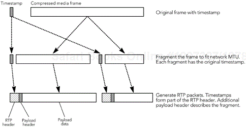
The fragmentation process is critical to the quality of the media in the presence of packet loss. The ability to decode each fragment independently is desirable; otherwise loss of a single fragment will result in the entire frame being discarded—a loss multiplier effect we wish to avoid. Payload formats that may require fragmentation typically define rules by which the payload data may be split in appropriate places, along with payload headers to help the receiver use the data in the event of some fragments being lost. These rules require support from the encoder to generate fragments that both obey the packing rules of the payload format and fit within the network MTU.
If the encoder cannot produce appropriately sized fragments, the sender may have to use an arbitrary fragmentation. Fragmentation can be accomplished by the application at the RTP layer, or by the network using IP fragmentation. If some fragments of an arbitrarily fragmented frame are lost, it is likely that the entire frame will have to be discarded, significantly impairing quality (Handley and Perkins33 describe these issues in more detail).
When multiple RTP packets are generated for each frame, the sender must choose between sending the packets in a single burst and spreading their transmission across the framing interval. Sending the packets in a single burst reduces the end-to-end delay but may overwhelm the limited buffering capacity of the network or receiving host. For this reason it is recommended that the sender spread the packets out in time across the framing interval. This issue is important mostly for high-rate senders, but it is good practice for other implementations as well.
In addition to the RTP header and the media data, packets often contain an additional payload-specific header. This header is defined by the RTP payload format specification in use, and provides an adaptation layer between RTP and the codec output.
Typical use of the payload header is to adapt codecs that were not designed for use over lossy packet networks to work on IP, to otherwise provide error resilience, or to support fragmentation. Well-designed payload headers can greatly enhance the performance of a payload format, and implementers should pay attention in order to correctly generate these headers, and to use the data provided to repair the effects of packet loss at the receiver.
The section titled Payload Headers in Chapter 4, RTP Data Transfer Protocol, discusses the use of payload headers in detail.
As highlighted in Chapter 1, An Introduction to RTP, a receiver is responsible for collecting RTP packets from the network, repairing and correcting for any lost packets, recovering the timing, decompressing the media, and presenting the result to the user. In addition, the receiver is expected to send reception quality reports so that the sender can adapt the transmission to match the network characteristics. The receiver will also typically maintain a database of participants in a session to be able to provide the user with information on the other participants. Figure 1.3 in Chapter 1 shows a block diagram of a receiver.
The first step of the reception process is to collect packets from the network, validate them for correctness, and insert them into a per-sender input queue. This is a straightforward operation, independent of the media format. The next section—Packet Reception—describes this process.
The rest of the receiver processing operates in a sender-specific manner and may be media-specific. Packets are removed from their input queue and passed to an optional channel-coding routine to correct for loss (Chapter 9 describes error correction). Following any channel coder, packets are inserted into a source-specific playout buffer, where they remain until complete frames have been received and any variation in interpacket timing caused by the network has been smoothed. The calculation of the amount of delay to add is one of the most critical aspects in the design of an RTP implementation and is explained in the section titled The Playout Buffer later in this chapter. The section titled Adapting the Playout Point describes a related operation: how to adjust the timing without disrupting playout of the media.
Sometime before their playout time is reached, packets are grouped to form complete frames, damaged or missing frames are repaired (Chapter 8, Error Concealment, describes repair algorithms), and frames are decoded. Finally, the media data is rendered for the user. Depending on the media format and output device, it may be possible to play each stream individually—for example, presenting several video streams, each in its own window. Alternatively, it may be necessary to mix the media from all sources into a single stream for playout—for example, combining several audio sources for playout via a single set of speakers. The final section of this chapter—Decoding, Mixing, and Playout—describes these operations.
The operation of an RTP receiver is a complex process, and more involved than the operation of a sender. This increased complexity is largely due to the variability inherent in IP networks: Most of the complexity comes from the need to compensate for lost packets and to recover the timing of a stream.
An RTP session comprises both data and control flows, running on distinct ports (usually the data packets flow on an even-numbered port, with control packets on the next higher—odd-numbered—port). This means that a receiving application will open two sockets for each session: one for data, one for control. Because RTP runs above UDP/IP, the sockets used are standard SOCK_DGRAM sockets, as provided by the Berkeley sockets API on UNIX-like systems, and by Winsock on Microsoft platforms.
Once the receiving sockets have been created, the application should prepare to receive packets from the network and store them for further processing. Many applications implement this as a loop, calling select() repeatedly to receive packets—for example:
fd_data = create_socket(...);
fd_ctrl = create_socket(...);
while (not_done) {
    FD_ZERO(&rfd);
    FD_SET(fd_data, &rfd);
    FD_SET(fd_ctrl, &rfd);
    timeout = ...;
    if (select(max_fd, &rfd, NULL, NULL, timeout) > 0) {
        if (FD_ISSET(fd_data, &rfd)) {
            ...validate data packet
            ...process data packet
        }
        if (FD_ISSET(fd_ctrl, &rfd)) {
            ...validate control packet
            ...process control packet
        }
    }
    ...do other processing
}
Data and control packets are validated for correctness as described in Chapters 4, RTP Data Transfer Protocol, and 5, RTP Control Protocol, and processed as described in the next two sections. The timeout of the select() operation is typically chosen according to the framing interval of the media. For example, a system receiving audio with 20-millisecond packet duration will implement a 20-millisecond timeout, allowing the other processing—such as decoding the received packets—to occur synchronously with arrival and playout, and resulting in an application that loops every 20 milliseconds.
Other implementations may be event driven rather than having an explicit loop, but the basic concept remains: Packets are continually validated and processed as they arrive from the network, and other application processing must be done in parallel to this (either explicitly time-sliced, as shown above, or as a separate thread), with the timing of the application driven by the media processing requirements. Real-time operation is essential to RTP receivers; packets must be processed at the rate they arrive, or reception quality will be impaired.
The first stage of the media playout process is to capture RTP data packets from the network, and to buffer those packets for further processing. Because the network is prone to disrupt the interpacket timing, as shown in Figure 6.5, there will be bursts when several packets arrive at once and/or gaps when no packets arrive, and packets may even arrive out of order. The receiver does not know when data packets are going to arrive, so it should be prepared to accept packets in bursts, and in any order.

As packets are received, they are validated for correctness, their arrival time is noted, and they are added to a per-sender input queue, sorted by RTP timestamp, for later processing. These steps decouple the arrival rate of packets from the rate at which they are processed and played to the user, allowing the application to cope with variation in the arrival rate. Figure 6.6 shows the separation between the packet reception and playout routines, which are linked only by the input queues.

It is important to store the exact arrival time, M, of RTP data packets so that the interarrival jitter can be calculated. Inaccurate arrival time measurements give the appearance of network jitter and cause the playout delay to increase. The arrival time should be measured according to a local reference wall clock, T, converted to the media clock rate, R. It is unlikely that the receiver has such a clock, so usually we calculate the arrival time by sampling the reference clock (typically the system wall clock time) and converting it to the local timeline:
where the offset is used to map from the reference clock to the media timeline, in the process correcting for skew between the media clock and the reference clock.
As noted earlier, processing of data packets may be time-sliced along with packet reception in a single-threaded application, or it may run in a separate thread in a multithreaded system. In a time-sliced design, a single thread handles both packet reception and playout. On each loop, all outstanding packets are read from the socket and inserted into the correct input queue. Packets are removed from the queues as needed and scheduled for playout. If packets arrive in bursts, some may remain in their input queue for multiple iterations of the loop, depending on the desired rate of playout and available processing capacity.
A multithreaded receiver typically has one thread waiting for data to arrive on the socket, sorting arriving packets onto the correct input queue. Other threads pull data from the input queues and arrange for the decoding and playout of the media. The asynchronous operation of the threads, along with the buffering in the input queues, effectively decouples the playout process from short-term variations in the input rate.
No matter what design is chosen, an application will usually not be able to receive and process packets continually. The input queues accommodate fluctuation in the playout process within the application, but what of delays in the packet reception routine? Fortunately, most general-purpose operating systems handle reception of UDP/IP packets on an interrupt-driven basis and can buffer packets at the socket level even when the application is busy. This capability provides limited buffering before packets reach the application. The default socket buffer is suitable for most implementations, but applications that receive high-rate streams or have significant periods of time when they are unable to handle reception may need to increase the size of the socket buffer beyond its default value (the setsockopt(fd, SOL_SOCKET, SO_RCVBUF, ...) function performs this operation on many systems). The larger socket buffer accommodates varying delays in packet reception processing, but the time packets spend in the socket buffer appears to the application as jitter in the network. The application might increase its playout delay to compensate for this perceived variation.
In parallel with the arrival of data packets, an application must be prepared to receive, validate, process, and send RTCP control packets. The information in the RTCP packets is used to maintain the database of the senders and receivers within a session, as discussed in Chapter 5, RTP Control Protocol, and for participant validation and identification, adaptation to network conditions, and lip synchronization. The participant database is also a good place from which to hang the participant-specific input queues, playout buffer, and other state needed by the receiver.
Single-threaded applications typically include both data and control sockets in their select() loop, interleaving reception of control packets along with all other processing. Multithreaded applications can devote a thread to RTCP reception and processing. Because RTCP packets are infrequent compared to data packets, the overhead of their processing is usually low and is not especially time-critical. It is, however, important to record the exact arrival time of sender report (SR) packets because this value is returned in receiver report (RR) packets and used in the round-trip time calculation.
When RTCP sender/receiver report packets arrive—describing the reception quality as seen at a particular receiver—the information they contain is stored. Parsing the report blocks in SR/RR packets is straightforward, provided you remember that the data is in network byte order and must be converted to host order before being used. The count field in the RTCP header indicates how many report blocks are present; remember that zero is a valid value, indicating that the sender of the RTCP packet is not receiving any RTP data packets.
The main use of RTCP sender/receiver reports is for an application to monitor reception of the streams it has sent: If the reports indicate poor reception, it is possible either to add error protection codes or to reduce the sending rate to compensate. In multisender sessions it is also possible to monitor the quality of other senders, as seen by other receivers; for example, a network operations center might monitor SR/RR packets as a check that the network is operating correctly. Applications typically store reception quality data as it is received, and periodically they use the stored data to adapt their transmission.
Sender reports also contain the mapping between the RTP media clock and the sender's reference clock, used for lip synchronization (see Chapter 7), and a count of the amount of data sent. Once again, this information is in network byte order and needs to be converted before use. This information needs to be stored if it is to be used for lip synchronization purposes.
When RTCP source description packets arrive, the information they contain is stored and may be displayed to the user. The RTP specification contains sample code to parse SDES packets (see Appendix A.5 of the specification50). The SDES CNAME (canonical name) provides the link between audio and video streams, indicating where lip synchronization should be performed. It is also used to group multiple streams coming from a single source—for example, if a participant has multiple cameras sending video to a single RTP session—and this may affect the way media is displayed to the user.
Once RTCP packets have been validated, the information they contain is added to the participant database. Because the validity checks for RTCP packets are strong, the presence of a participant in the database is a solid indication that the participant is valid. This is a useful check when RTP packets are being validated: If the SSRC in an RTP data packet was previously seen in an RTCP packet, it is highly likely to be a valid source.
When RTCP BYE packets are received, entries in the participant database are marked for later removal. As noted in Chapter 5, RTP Control Protocol, entries are not removed immediately but should be kept for some small time to allow any delayed packets to arrive. (My own implementation uses a fixed two-second timeout; the precise value is unimportant, provided that it is larger than the typical network timing jitter.) Receivers also perform periodic housekeeping to time out inactive participants. Performing this task with every packet is not necessary; once per RTCP report interval is sufficient.
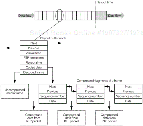
Data packets are extracted from their input queue and inserted into a source-specific playout buffer sorted by their RTP timestamps. Frames are held in the playout buffer for a period of time to smooth timing variations caused by the network. Holding the data in a playout buffer also allows the pieces of fragmented frames to be received and grouped, and it allows any error correction data to arrive. The frames are then decompressed, any remaining errors are concealed, and the media is rendered for the user. Figure 6.7 illustrates the process.

A single buffer may be used to compensate for network timing variability and as a decode buffer for the media codec. It is also possible to separate these functions: using separate buffers for jitter removal and decoding. However, there is no strict layering requirement in RTP: Efficient implementations often mingle related functions across layer boundaries, a concept termed integrated layer processing.65
The playout buffer comprises a time-ordered linked list of nodes. Each node represents a frame of media data, with associated timing information. The data structure for each node contains pointers to the adjacent nodes, the arrival time, RTP timestamp, and desired playout time for the frame, and pointers to both the compressed fragments of the frame (the data received in RTP packets) and the uncompressed media data. Figure 6.8 illustrates the data structures involved.
When the first RTP packet in a frame arrives, it is removed from the input queue and positioned in the playout buffer in order of its RTP timestamp. This involves creating a new playout buffer node, which is inserted into the linked list of the playout buffer. The compressed data from the recently arrived packet is linked from the playout buffer node, for later decoding. The frame's playout time is then calculated, as explained later in this chapter.
The newly created node resides in the playout buffer until its playout time is reached. During this waiting period, packets containing other fragments of the frame may arrive and are linked from the node. Once it has been determined that all the fragments of a frame have been received, the decoder is invoked and the resulting uncompressed frame linked from the playout buffer node. Determining that a complete frame has been received depends on the codec:
Audio codecs typically do not fragment frames, and they have a single packet per frame (MPEG Audio Layer-3—MP3—is a common exception);
Video codecs often generate multiple packets per video frame, with the RTP marker bit being set to indicate the RTP packet containing the last fragment.
The decision of when to invoke the decoder depends on the receiver and is not specified by RTP. Frames can be decoded as soon as they arrive or kept compressed until the last possible moment. The choice depends on the relative availability of processing cycles and storage space for uncompressed frames, and perhaps on the receiver's estimate of future resource availability. For example, a receiver may wish to decode data early if it knows that an index frame is due and it will shortly be busy.
Eventually the playout time for a frame arrives, and the frame is queued for playout as discussed in the section Decoding, Mixing, and Playout later in this chapter. If the frame has not already been decoded, at this time the receiver must make its best effort to decode the frame, even if some fragments are missing, because this is the last chance before the frame is needed. This is also the time when error concealment (see Chapter 8) may be invoked to hide any uncorrected packet loss.
Once the frame has been played out, the corresponding playout buffer node and its linked data should be destroyed or recycled. If error concealment is used, however, it may be desirable to delay this process until the surrounding frames have also been played out because the linked media data may be useful for the concealment operation.
RTP packets arriving late and corresponding to frames that have missed their playout point should be discarded. The timeliness of a packet can be determined by comparison of its RTP timestamp with the timestamp of the oldest packet in the playout buffer (note that the comparison should be done with 32-bit modulo arithmetic, to allow for timestamp wrap-around). It is clearly desirable to choose the playout delay so that late packets are rare, and applications should monitor the number of late packets and be prepared to adapt their playout delay in response. Late packets indicate an inappropriate playout delay, typically caused by changing network delays or skew between clocks at the sending and receiving hosts.
The trade-off in playout buffer operation is between fidelity and delay: An application must decide the maximum playout delay it can accept, and this in turn determines the fraction of packets that arrive in time to be played out. A system designed for interactive use—for example, video conferencing or telephony—must try to keep the playout delay as small as possible because it cannot afford the latency incurred by the buffering. Studies of human perception point to a limit in round-trip time of about 300 milliseconds as the maximum tolerable for interactive use; this limit implies an end-to-end delay of only 150 milliseconds including network transit time and buffering delay if the system is symmetric. However, a noninteractive system, such as streaming video, television, or radio, may allow the playout buffer to grow up to several seconds, thereby enabling noninteractive systems to handle variation in packet arrival times better.
The main difficulty in designing an RTP playout buffer is determining the playout delay: How long should packets remain in the buffer before being scheduled for playout? The answer depends on various factors:
The delay between receiving the first and last packets of a frame
The delay before any error correction packets are received (see Chapter 9, Error Correction)
The variation in interpacket timing caused by network queuing jitter and route changes
The relative clock skew between sender and receiver
The end-to-end delay budget of the application, and the relative importance of reception quality and latency
The factors under control of the application include the spacing of packets in a frame, and the delay between the media data and any error correction packets, both of which are controlled by the sender. The effects of these factors on the playout delay calculation are discussed in the section titled Compensation for Sender Behavior later in this chapter.
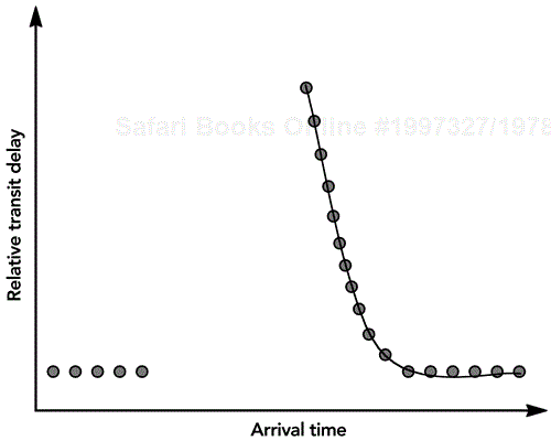
Outside the control of the application is the behavior of the network, and the accuracy and stability of the clocks at sender and receiver. As an example, consider Figure 6.9, which shows the relationship between packet transmission time and reception time for a trace of RTP audio packets. If the sender clock and receiver clock run at the same rate, as is desired, the slope of this plot should be exactly 45 degrees. In practice, sender and receiver clocks are often unsynchronized and run at slightly different rates. For the trace in Figure 6.9, the sender clock is running faster than the receiver clock, so the slope of the plot is less than 45 degrees (Figure 6.9 is an extreme example, to make it easy to see the effect; the slope is typically much closer to 45 degrees). The section titled Compensation for Clock Skew later in this chapter explains how to correct for unsynchronized clocks.

If the packets have a constant network transit time, the plot in Figure 6.9 will produce an exactly straight line. However, typically the network induces some jitter in the interpacket spacing due to variation in queuing delays, and this is observable in the figure as deviations from the straight-line plot. The figure also shows a discontinuity, resulting from a step change in the network transit time, most likely due to a route change in the network. Chapter 2, Voice and Video Communication over Packet Networks, has a more detailed discussion of the effects, and the section titled Compensation for Jitter later in this chapter explains how to correct for these issues. Correcting for more extreme variations is discussed in the sections Compensation for Route Changes and Compensation for Packet Reordering.
The final point to consider is the end-to-end delay budget of the application. This is mainly a human-factors issue: What is the maximum acceptable end-to-end delay for the users of the application, and how long does this leave for smoothing in the playout buffer after the network transit time has been factored out? As might be expected, the amount of time available for buffering does affect the design of the playout buffer; the section titled Compensation for Jitter discusses this subject further.
A receiver should take these factors into account when determining the playout time for each frame. The playout calculation follows several steps:
The sender timeline is mapped to the local playout timeline, compensating for the relative offset between sender and receiver clocks, to derive a base time for the playout calculation (see Mapping to the Local Timeline later in this chapter).
If necessary, the receiver compensates for clock skew relative to the sender, by adding a skew compensation offset that is periodically adjusted to the base time (see Compensation for Clock Skew).
The playout delay on the local timeline is calculated according to a sender-related component of the playout delay (see Compensation for Sender Behavior) and a jitter-related component (see Compensation for Jitter).
The playout delay is adjusted if the route has changed (see Compensation for Route Changes), if packets have been reordered (see Compensation for Packet Reordering), if the chosen playout delay causes frames to overlap, or in response to other changes in the media (see Adapting the Playout Point).
Finally, the playout delay is added to the base time to derive the actual playout time for the frame.
Figure 6.10 illustrates the playout calculation, noting the steps of the process. The following sections give details of each stage.

The first stage of the playout calculation is to map from the sender's timeline (as conveyed in the RTP timestamp) to a time-line meaningful to the receiver, by adding the relative offset between sender and receiver clocks to the RTP timestamp.
To calculate the relative offset, the receiver tracks the difference, d(n), between the RTP timestamp of the nth packet, TR(n), and the arrival time of that packet, TL(n), measured in the same units:
The difference, d(n), includes a constant factor because the sender and receiver clocks were initialized at different times with different random values, a variable delay due to data preparation time at the sender, a constant factor due to the minimum network transit time, a variable delay due to network timing jitter, and a rate difference due to clock skew. The difference is a 32-bit unsigned integer, like the timestamps from which it is calculated; and because the sender and receiver clocks are unsynchronized, it can have any 32-bit value.
The difference is calculated as each packet arrives, and the receiver tracks its minimum observed value to obtain the relative offset:
Because of the rate difference between TL(n) and TR(n) due to clock skew, the difference, d(n), will tend to drift larger or smaller. To prevent this drift, the minimum offset is calculated over a window, w, of the differences since the last compensation for clock skew. Also note that an unsigned comparison is required because the values may wrap around:
The offset value is used to calculate the base playout point, according to the timeline of the receiver:
This is the initial estimate of the playout time, to which are applied additional factors compensating for clock skew, jitter, and so on.
RTP payload formats define the nominal clock rate for a media stream but place no requirements on the stability and accuracy of the clock. Sender and receiver clocks commonly run at slightly different rates, forcing the receiver to compensate for the variation. A plot of packet transmission time versus reception time, as in Figure 6.9, illustrates this. If the slope of the plot is exactly 45 degrees, the clocks have the same rate; deviations are caused by clock skew between sender and receiver.
Receivers must detect the presence of clock skew, estimate its magnitude, and adjust the playout point to compensate. There are two possible compensation strategies: tuning the receiver clock to match the sender clock, or periodically adjusting playout buffer occupancy to regain alignment.
The latter approach accepts the skew and periodically realigns the playout buffer by inserting or deleting data. If the sender is faster, the receiver will eventually have to discard some data to bring the clocks into alignment, otherwise its playout buffer will be over-run. If the sender is slower, the receiver will eventually run out of media to play, and must synthesize some data to fill the gap that is left. The magnitude of the clock skew determines the frequency of playout point adjustments, and hence the quality degradation experienced.
Alternatively, if the receiver clock rate is finely adjustable, it may be possible to tune its rate to exactly match that of the sender, avoiding the need for a playout buffer realignment. This approach can give higher quality because data is never discarded due to skew, but it may require hardware support that is not common (systems using audio may be able to resample to match the desired rate using software).
Estimating the amount of clock skew present initially appears to be a simple problem: Observe the rate of the sender clock—the RTP timestamp—and compare with the local clock. If TR(n) is the RTP timestamp of the nth packet received, and TL(n) is the value of the local clock at that time, then the clock skew can be estimated as follows:
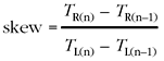
with a skew of less than unity meaning that the sender is slower than the receiver, and a skew of greater than unity meaning that the sender clock is fast compared to the receiver. Unfortunately, the presence of network timing jitter means that this simple estimate is not sufficient; it will be directly affected by variation in interpacket spacing due to jitter. Receivers must look at the long-term variation in the packet arrival rate to derive an estimate for the underlying clock skew, removing the effects of jitter.
There are many possible algorithms for managing clock skew, depending on the accuracy and sensitivity to jitter that is required. In the following discussion I describe a simple approach to estimating and compensating for clock skew that has proven suitable for voice-over-IP applications,79 and I give pointers to algorithms for more demanding applications.
The simple approach to clock skew management continually monitors the average network transit delay and compares it with an active delay estimate. Increasing divergence between the active delay estimate and measured average delay denotes the presence of clock skew, eventually causing the receiver to adapt playout. As each packet arrives, the receiver calculates the instantaneous one-way delay for the nth packet, dn, based on the reception time of the packet and its RTP timestamp:
On receipt of the first packet, the receiver sets the active delay, E = d0, and the estimated average delay, D0 = d0. With each subsequent packet the average delay estimate, Dn, is updated by an exponentially weighted moving average:
The factor 31/32 controls the averaging process, with values closer to unity making the average less sensitive to short-term fluctuation in the transit time. Note that this calculation is similar to the calculation of the estimated jitter; but it retains the sign of the variation, and it uses a time constant chosen to capture the long-term variation and reduce the response to short-term jitter.
The average one-way delay, Dn, is compared with the active delay estimate, E, to estimate the divergence since the last estimate:
If the sender clock and receiver clock are synchronized, the divergence will be close to zero, with only minor variations due to network jitter. If the clocks are skewed, the divergence will increase or decrease until it exceeds a predetermined threshold, causing the receiver to take compensating action. The threshold depends on the jitter, the codec, and the set of possible adaptation points. It has to be large enough that false adjustments due to jitter are avoided, and it should be chosen such that the discontinuity caused by an adjustment can easily be concealed. Often a single framing interval is suitable, meaning that an entire codec frame is inserted or removed.
Compensation involves growing or shrinking the playout buffer as described in the section titled Adapting the Playout Point later in this chapter. The playout point can be changed up to the divergence as measured in RTP timestamp units (for audio, the divergence typically gives the number of samples to add or remove). After compensating for skew, the receiver resets the active delay estimate, E, to equal the current delay estimate, Dn, resetting the divergence to zero in the process (the estimate for base_play-out_time(n) is also reset at this time).
In C-like pseudocode, the algorithm performed as each packet is received becomes this:
adjustment_due_to_skew(rtp_packet p, uint32_t curr_time) {
    static int       first_time = 1;
    static uint32_t  delay_estimate;
    static uint32_t  active_delay;
    uint32_t         adjustment = 0;
    uint32_t         d_n = p->ts – curr_time;

    if (first_time) {
        first_time = 0;
        delay_estimate = d_n;
        active_delay = d_n;
    } else {
        delay_estimate = (31 * delay_estimate + d_n)/32;
    }
    if (active_delay – delay_estimate > SKEW_THRESHOLD) {
        // Sender is slow compared to receiver
        adjustment   = SKEW_THRESHOLD;
        active_delay = delay_estimate;
    }
    if (active_delay – delay_estimate < -SKEW_THRESHOLD) {
        // Sender is fast compared to receiver
        adjustment   = -SKEW_THRESHOLD;
        active_delay = delay_estimate;
    }
    // Adjustment will be 0, SKEW_THRESHOLD, or –SKEW_THRESHOLD. It is
    // appropriate that SKEW_THRESHOLD equals the framing interval.
    return adjustment;
}
The assumptions of this algorithm are that the jitter distribution is symmetric and that any systematic bias is due to clock skew. If the distribution of skew values is asymmetric for reasons other than clock skew, this algorithm will cause spurious skew adaptation. Significant short-term fluctuations in the network transit time also might confuse the algorithm, causing the receiver to perceive network jitter as clock skew and adapt its playout point. Neither of these issues should cause operational problems: The skew compensation algorithm will eventually correct itself, and any adaptation steps would likely be needed in any case to accommodate the fluctuations.
Another assumption of the skew compensation described here is that it is desirable to make step adjustments to the playout point—for example, adding or removing a complete frame at a time—while concealing the discontinuity as if a packet were lost. For many codecs—in particular, frame-based voice codecs—this is appropriate behavior because the codec is optimized to conceal lost frames and skew compensation can leverage this ability, provided that care is taken to add or remove unimportant, typically low-energy, frames. In some cases, however, it is desirable to adapt more smoothly, perhaps interpolating a single sample at a time.
If smoother adaptation is needed, the algorithm by Moon et al.90 may be more suitable, although it is more complex and has correspondingly greater requirements for state maintenance. The basis of their approach is to use linear programming on a plot of observed one-way delay versus time, to fit a line that lies under all the data points, as closely to them as possible. An equivalent approach is to derive a best-fit line under the data points of a plot such as that in Figure 6.9, and use this to estimate the slope of the line, and hence the clock skew. Such algorithms are more accurate, provided the skew is constant, but they clearly have higher overheads because they require the receiver to keep a history of points, and perform an expensive line-fitting algorithm. They can, however, derive very accurate skew measurements, given a long enough measurement interval.
Long-running applications should take into account the possibility that the skew might be nonstationary, and vary according to outside effects. For example, temperature changes can affect the frequency of crystal oscillators and cause variation in the clock rate and skew between sender and receiver. Nonstationary clock skew may confuse some algorithms (for example, that of Moon et al.90) that use long-term measurements. Other algorithms, such as that of Hodson et al.,79 described earlier, work on shorter timescales and periodically recalculate the skew, so they are robust to variations.
When choosing a clock skew estimation algorithm, it is important to consider how the playout point will be varied, and to choose an estimator with an appropriate degree of accuracy. For example, applications using frame-based audio codecs may adapt by adding or removing a single frame, so an estimator that measures skew to the nearest sample may be overkill. The section titled Adapting the Playout Point later in this chapter discusses this issue in more detail.
The nature of the sender's packet generation process can influence the receiver's playout calculation in several ways, causing increased playout buffering delay.
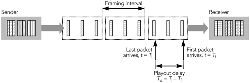
If the sender spreads the packets that make up a frame in time across the framing interval, as is common for video, there will be a delay between the first and last packets of a frame, and receivers must buffer packets until the whole frame is received. Figure 6.11 shows the insertion of additional playout delay, Td, to ensure that the receiver does not attempt to play out the frame before all the fragments have arrived.
If the interframe timing and number of packets per frame are known, inserting this additional delay is simple. Assuming that the sender spaces packets evenly, the adjustment will be as follows:
adjustment_due_to_fragmentation = (packets_per_frame – 1)
                            × (interframe_time / packets_per_frame)
Unfortunately, receivers do not always know these variables in advance. For example, the frame rate may not be signaled during session setup, the frame rate may vary during a session, or the number of packets per frame may vary during a session. This variability can make it difficult to schedule playout because it is unclear how much delay needs to be added to allow all fragments to arrive. The receiver must estimate the required playout delay, and adapt if the estimate proves inaccurate.
The estimated playout compensation could be calculated by a special-purpose routine that looked at the arrival times of fragments to calculate an average fragmentation delay. Fortunately, this is not necessary; the jitter calculation performs the same role. All packets of a frame have the same timestamp—representing the time of the frame, rather than the time the packet was sent—so fragmented frames cause the appearance of jitter (the receiver cannot differentiate between a packet delayed in the network and one delayed by the sender). The strategies for jitter compensation discussed in the next section can therefore be used to estimate the amount of buffering delay needed to compensate for fragmentation, and there is no need to account for fragmentation in the host component of the playout delay.
Similar issues arise if the sender uses the error correction techniques described in Chapter 9. For error correction packets to be useful, playout must be delayed so that the error correction packets arrive in time to be used. The presence of error correction packets is signaled during session setup, and the signaling may include enough information to allow the receiver to size the playout buffer correctly. Alternatively, the correct playout delay must be inferred from the media stream. The compensation delay needed depends on the type of error correction employed. Three common types of error correction are parity FEC (forward error correction), audio redundancy, and retransmission.
The parity FEC scheme discussed in Chapter 932 leaves the data packets unmodified, and sends error correction packets in a separate RTP stream. The error correction packets contain a bit mask in their FEC header to identify the sequence numbers of the packets they protect. By observing the mask, a receiver can determine the delay to add, in packets. If packet spacing is constant, this delay translates to a time offset to add to the playout calculation. If the interpacket spacing is not constant, the receiver must use a conservative estimate of the spacing to derive the required play-out delay.
The audio redundancy scheme10 discussed in Chapter 9, Error Correction, includes a time offset in redundant packets, and this offset may be used to size the playout buffer. At the start of a talk spurt, redundant audio may be used in two modes: Initial packets may be sent without the redundancy header, or they may be sent with a zero-length redundant block. As Figure 6.12 shows, sizing the playout buffer is easier if a zero-length redundant block is included with initial packets in a talk spurt. Unfortunately, including these blocks is not mandatory in the specification, and implementations may have to guess an appropriate playout delay if it is not present (a single packet offset is most common and makes a reasonable estimate in the absence of other information). Once a media stream has been determined to use redundancy, the offset should be applied to all packets in that stream, including any packets sent without redundancy at the beginning of a talk spurt. If a complete talk spurt is received without redundancy, it can be assumed that the sender has stopped redundant transmission, and future talk spurts can be played without delay.

A receiver of either parity FEC or redundancy should initially pick a large playout delay, to ensure that any data packets that arrive are buffered. When the first error correction packet arrives, it will cause the receiver to reduce its playout delay, reschedule, and play out any previously buffered packets. This process avoids a gap in playout caused by an increase in buffering delay, at the expense of slightly delaying the initial packet.
When packet retransmission is used, the playout buffer must be sized larger than the round-trip time between sender and receiver, to allow time for the retransmission request to return to the sender and be serviced. The receiver has no way of knowing the roundtrip time, short of sending a retransmission request and measuring the response time. This does not affect most implementations because retransmission is typically used in noninteractive applications in which the playout buffering delay is larger than the round-trip time, but it may be an issue if the round-trip time is large.
No matter what error correction scheme is used, the sender may be generating an excessive amount of error correction data. For example, when sending to a multicast group, the sender might choose an error correction code based on the worst-case receiver, which will be excessive for other receivers. As noted by Rosen-berg et al.,101 it may then be possible to repair some fraction of loss with only a subset of the error correction data. In this case a receiver may choose a playout delay smaller than that required for all of the error correction data, instead just waiting long enough to repair the loss it chooses. The decision to ignore some error correction data is made solely by the receiver and based on its view of the transmission quality.
Finally, if the sender interleaves the media stream—as will be described in Chapter 8, Error Concealment—the receiver must allow for this in the playout calculation so that it can sort interleaved packets into playout order. Interleaving parameters are typically signaled during session setup, allowing the receiver to choose an appropriate buffering delay. For example, the AMR payload format41 defines an interleaving parameter that can be signaled in the SDP a=fmtp: line, denoting the number of packets per interleaving group (and hence the amount of delay in terms of the number of packets that should be inserted into the playout buffer to compensate). Other codecs that support interleaving should supply a similar parameter.
To summarize, the sender may affect the playout buffer in three ways: by fragmenting frames and delaying sending fragments, by using error correction packets, or by interleaving. The first of these will be compensated for according to the usual jitter compensation algorithm; the others require the receiver to adjust the playout buffer to compensate. This compensation is mostly an issue for interactive applications that use small playout buffers to reduce latency; streaming media systems can simply set a large playout buffer.
When RTP packets flow over a real-world IP network, variation in the interpacket timing is inevitable. This network jitter can be significant, and a receiver must compensate by inserting delay into its playout buffer so that packets held up by the network can be processed. Packets that are delayed too much arrive after their playout time has passed and are discarded; with suitable selection of a playout algorithm, this should be a rare occurrence. Figure 6.13 shows the jitter compensation process.

There is no standard algorithm for calculation of the jitter compensation delay; most applications will want to calculate the play-out delay adaptively and may use different algorithms, depending on the application type and network conditions. Applications that are designed for noninteractive scenarios would do well to pick a compensation delay significantly larger than the expected jitter; an appropriate value might be several seconds. More complex is the interactive case, in which the application desires to keep the play-out delay as small as possible (values on the order of tens of milliseconds are not unrealistic, given network and packetization delays). To minimize the playout delay, it is necessary to study the properties of the jitter and use these to derive the minimum suitable playout delay.
In many cases the network-induced jitter is essentially random. A plot of interpacket arrival times versus frequency of occurrence will, in this case, be somewhat similar to the Gaussian distribution shown in Figure 6.14. Most packets are only slightly affected by the network jitter, but some outliers are significantly delayed or are back-to-back with a neighboring packet.

How accurate is this approximation? That depends on the network path, of course, but measurements taken by me and by Moon et al.91 show that the approximation is reasonable in many cases, although real-world data is often skewed toward larger interarrival times and has a sharp minimum cutoff value (as illustrated by the “actual distribution” in Figure 6.14). The difference is usually not critical, because the number of packets in the discard region is small.
If it can be assumed that the jitter distribution does approximate a Gaussian normal distribution, then deriving a suitable playout delay is easily possible. The standard deviation of the jitter is calculated, and from probability theory we know that more than 99% of a normal distribution lies within three times the standard deviation of the mean (average) value. An implementation could choose a playout delay that is equal to three times the standard deviation in interarrival times and expect to discard less than 0.5% of packets because of late arrival. If this delay is too long, using a playout delay of twice the standard deviation will give an expected discard rate due to late arrival of less than 2.5%, again because of probability theory.
How can we measure the standard deviation? The jitter value calculated for insertion into RTCP receiver reports tracks the average variation in network transit time, which can be used to approximate the standard deviation. On the basis of these approximations, the playout delay required to compensate for network jitter can be estimated as three times the RTCP jitter estimate for a particular source. The playout delay for a new frame is set to at least
Tplayout = Tcurrent + 3J
where J is the current estimate of the jitter, as described in Chapter 5, RTP Control Protocol. The value of Tplayout may be modified in a media-dependent manner, as discussed later. Implementations using this value as a base for their playout calculation have shown good performance in a range of real-world conditions.
The jitter distribution depends both on the path that traffic takes through the network and on the other traffic sharing that path. The primary cause of jitter is competition with other traffic, resulting in varying queuing delays at the intermediate routers; clearly, changes in the other traffic also will affect the jitter seen by a receiver. For this reason receivers should periodically recalculate the amount of playout buffering delay they use, in case the network behavior has changed, adapting if necessary. When should receivers adapt? This is not a trivial question, because any change in the playout delay while the media is playing will disrupt the playout, causing either a gap where there is nothing to play, or forcing the receiver to discard some data to make up lost time. Accordingly, receivers try to limit the number of times they adapt their playout point. Several factors can be used as triggers for adaptation:
A significant change in the fraction of packets discarded because of late arrival
Receipt of several consecutive packets that must be discarded because of late arrival (three consecutive packets is a suitable threshold)
Receipt of packets from a source that has been inactive for a long period of time (ten seconds is a suitable threshold)
The onset of a spike in the network transit delay
With the exception of spikes in the network transit delay, these factors should be self-explanatory. As shown in Figure 2.12 in Chapter 2, Voice and Video Communication over Packet Networks, the network occasionally causes “spikes” in the transit delay, when several packets are delayed and arrive in a burst. Such spikes can easily bias a jitter estimate, causing the application to choose a larger playout delay than is required. In many applications this increase in playout delay is acceptable, and applications should treat a spike as any other form of jitter and increase their playout delay to compensate. However, some applications prefer increased packet loss to increased latency; these applications should detect the onset of a delay spike and ignore packets in the spike when calculating the playout delay.91,96
Detecting the start of a delay spike is simple: If the delay between consecutive packets increases suddenly, a delay spike likely has occurred. The scale of a “sudden increase” is open to some interpretation: Ramjee et al.96 suggest that twice the statistical variance in interarrival time, plus 100 milliseconds, is a suitable threshold; another implementation that I'm familiar with uses a fixed threshold of 375 milliseconds (both are voice-over-IP systems using 8kHz speech).
Once a delay spike has been detected, an implementation should suspend normal jitter adjustment until the spike has ended. As a result, several packets will probably be discarded because of late arrival, but it is assumed that the application has a strict delay bound, and that this result is preferable to an increased playout delay.
Locating the end of a spike is harder than detecting the onset. One key characteristic of a delay spike is that packets that were evenly spaced at the sender arrive in a burst after the spike, meaning that each packet has a progressively smaller transit delay, as shown in Figure 6.15. The receiver should maintain an estimate of the “slope” of the spike, and once it is sufficiently close to flat, the spike can be assumed to have ended.
Given all these factors, pseudocode to compensate playout delay for the effects of jitter and delay spikes is as follows:
int
adjustment_due_to_jitter(...)
{
    delta_transit = abs(transit – last_transit);
    if (delta_transit > SPIKE_THRESHOLD) {
        // A new "delay spike" has started
        playout_mode = SPIKE;
        spike_var = 0;
        adapt = FALSE;
    } else {
        if (playout_mode == SPIKE) {
            // We're within a delay spike; maintain slope estimate
            spike_var = spike_var / 2;
            delta_var = (abs(transit – last_transit) + abs(transit
                                             last_last_transit))/8;
            spike_var = spike_var + delta_var;
            if (spike_var < spike_end) {
                // Slope is flat; return to normal operation
                playout_mode = NORMAL;
            }
            adapt = FALSE;
        } else {
            // Normal operation; significant events can cause us to
            //adapt the playout
            if (consecutive_dropped > DROP_THRESHOLD) {
                // Dropped too many consecutive packets
                adapt = TRUE;
            }
            if ((current_time – last_header_time) >
                                              INACTIVE_THRESHOLD) {
                // Silent source restarted; network conditions have
                //probably changed
                adapt = TRUE;
            }
        }
    }
    desired_playout_offset = 3 * jitter
    if (adapt) {
        playout_offset = desired_playout_offset;
    } else {
        playout_offset = last_playout_offset;
    }
    return playout_offset;
}
The key points are that jitter compensation is suspended during a delay spike, and that the actual playout time changes only when a significant event occurs. At other times the desired_playout_offset is stored to be instated at a media-specific time (see the section titled Adapting the Playout Point).
Although infrequent, route changes can occur in the network because of link failures or other topology changes. If a change occurs in the route taken by the RTP packets, it will manifest itself as a sudden change in the network transit time. This change will disrupt the playout buffer because either the packets will arrive too late for playout, or they will be early and overlap with previous packets.
The jitter and delay spike compensation algorithms should detect the change in delay and adjust the playout to compensate, but this approach may not be optimal. Faster adaptation can take place if the receiver observes the network transit time directly and adjusts the playout delay in response to a large change. For example, an implementation might adjust the playout delay if the transit delay changes by more than five times the current jitter estimate. The relative network transit time is used as part of the jitter calculation, so such observation is straightforward.
In extreme cases, jitter or route changes can result in packets being reordered in the network. As discussed in Chapter 2, Voice and Video Communication over Packet Networks, this is usually a rare occurrence, but it happens frequently enough that implementations need to be able to compensate for its effects and smoothly play out a media stream that contains out-of-order packets.
Reordering should not be an issue for correctly designed receivers: Packets are inserted into the playout buffer according to their RTP timestamp, irrespective of the order in which they arrive. If the playout delay is sufficiently large, they are played out in their correct sequence; otherwise they are discarded as any other late packet. If many packets are discarded because of reordering and late arrival, the standard jitter compensation algorithm will take care of adjusting the playout delay.
There are two basic approaches to adapting the playout point: receivers can either slightly adjust the playout time for each frame, making continual small adjustments to the playout point, or they can insert or remove complete frames from the media stream, making a smaller number of large adjustments as they become necessary. No matter how the adjustment is made, the media stream is disrupted to some extent. The aim of the adaptation must be to minimize this disruption, which requires knowledge of the media stream; accordingly, audio and video playout adaptation strategies are discussed separately.
Audio is a continuous media format, meaning that each audio frame occupies a certain amount of time, and the next is scheduled to start immediately after it finishes. There are no gaps between frames unless silence suppression is used, and hence there is no convenient time to adapt the playout delay. For this reason the presence of silence suppression has a significant effect on the design of audio playout buffer algorithms.
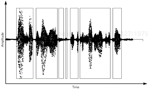
For conversational speech signals, an active speaker will generate talk spurts several hundred milliseconds in duration, separated by silent periods. Figure 6.16 shows the presence of talk spurts in a speech signal, and the gaps left between them. The sender detects frames representing silent periods and suppresses the RTP packets that would otherwise be generated for those frames. The result is a sequence of packets with consecutive sequence numbers, but a jump in the RTP timestamp depending on the length of the silent period.
Adjusting the playout point during a talk spurt will cause an audible glitch in the output, but a small change in the length of the silent period between talk spurts will not be noticeable.92 This is the key point to remember in the design of a playout algorithm for an audio tool: If possible, adjust the playout point only during silent periods.
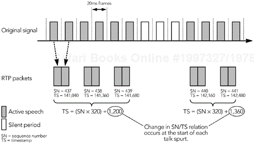
It is usually a simple matter for a receiver to detect the start of a talk spurt, because the sender is required to set the marker bit on the first packet after a silent period, providing an explicit indication of the start of a talk spurt. Sometimes, however, the first packet in a talk spurt is lost. It is usually still possible to detect that a new talk spurt has started, because the sequence number/timestamp relationship will change as shown in Figure 6.17, providing an implicit indication of the start of the talk spurt.
Once the start of the talk spurt has been located, you may adjust the playout point by slightly changing the length of the silent period. The playout delay is then held constant for all of the packets in the talk spurt. The appropriate playout delay is calculated during each talk spurt and used to adapt the playout point for the following talk spurt, under the assumption that conditions are unlikely to change significantly between talk spurts.
Some speech codecs send low-rate comfort noise frames during silent periods so that the receiver can play appropriate background noise to achieve a more pleasant listening experience. The receipt of a comfort noise packet indicates the end of a talk spurt and a suitable time to adapt the playout delay. The length of the comfort noise period can be varied without significant effects on the audio quality. The RTP payload type does not usually indicate the comfort noise frames, so it is necessary to inspect the media data to detect their presence. Older codecs that do not have native comfort noise support may use the RTP payload format for comfort noise,42 which is indicated by RTP payload type 13.
In exceptional cases it may be necessary to adapt during a talk spurt—for example, if multiple packets are being discarded because of late arrival. These cases are expected to be rare because talk spurts are relatively short and network conditions generally change slowly.
Combining these features produces pseudocode to determine an appropriate time to adjust the playout point, assuming that silence suppression is used, as follows:
int
should_adjust_playout(rtp_packet curr, rtp_packet prev, int contdrop) {
    if (curr->marker) {
        return TRUE; // Explicit indication of new talk spurt
    }
    delta_seq = curr->seq – prev->seq;
    delta_ts = curr->ts - prev->ts;
    if (delta_seq * inter_packet_gap != delta_ts) {
        return TRUE; // Implicit indication of new talk spurt
    }
    if (curr->pt == COMFORT_NOISE_PT) || is_comfort_noise(curr)) {
        return TRUE; // Between talk spurts
    }
    if (contdrop > CONSECUTIVE_DROP_THRESHOLD) {
        contdrop = 0;
        return TRUE; // Something has gone badly wrong, so adjust
    }
    return FALSE;
}
The variable contdrop counts the number of consecutive packets discarded because of inappropriate playout times—for example, if a route change causes packets to arrive too late for playout. An appropriate value for CONSECUTIVE_DROP_THRESHOLD is three packets.
If the function should_adjust_playout() returns TRUE, the receiver is either in a silent period or has miscalculated the playout point. If the calculated playout point has diverged from the currently used value, it should adjust the playout points for future packets, by changing their scheduled playout time. There is no need to generate fill-in data, only to continue playing silence/comfort noise until the next packet is scheduled (this is true even when adjustment has been triggered by multiple consecutive packet drops because this indicates that playout has stopped).
Care needs to be taken when the playout delay is being reduced because a significant change in conditions could bring the start of the next talk spurt so far forward that it would overlap with the end of the previous talk spurt. The amount of adaptation that may be performed is thus limited, because clipping the start of a talk spurt is not desirable.
When receiving audio transmitted without silence suppression, the receiver must adapt the playout point while audio is being played out. The most desirable means of adaptation is tuning the local media clock to match that of the transmitter so that data can be played out directly. If this is not possible, because the necessary hardware support is lacking, the receiver will have to vary the playout point either by generating fill-in data to be inserted into the media stream or by removing some media data from the playout buffer. Either approach inevitably causes some disruption to the playout, and it is important to conceal the effects of adaptation to ensure that it does not disturb the listener.
There are several possible adaptation algorithms, depending on the nature of the output device and the resources of the receiver:
The audio can be resampled in software to match the rate of the output device. A standard signal-processing text will provide various algorithms, depending on the desired quality and resource trade-off. This is a good, general-purpose solution.
Sample-by-sample adjustments in the playout delay can be made on the basis of knowledge of the media content. For example, Hodson et al.79 use a pattern-matching algorithm to detect pitch cycles in speech that are removed or duplicated to adapt the playout (pitch cycles are much shorter than complete frames, so this approach gives fine-grained adaptation). This approach can perform better than resampling, but it is highly content-specific.
Complete frames can be inserted or deleted, as if packets were lost or duplicated. This algorithm is typically not of high quality, but it may be required if a hardware decoder designed for synchronous networks is used.
In the absence of silence suppression, there is no obvious time to adjust the playout point. Nevertheless, a receiver can still make intelligent choices regarding playout adaptation, by varying the playout at times where error concealment is more effective—for example, during a period of relative quiet or a period during which the signal is highly repetitive—depending on the codec and error concealment algorithm. Loss concealment strategies are described in detail in Chapter 8, Error Concealment.
Video is a discrete media format in which each frame samples the scene at a particular instant in time and the interval between frames is not recorded. The discrete nature of video provides flexibility in the playout algorithm, allowing the receiver to adapt the playout by slightly varying the interframe timing. Unfortunately, display devices typically operate at a fixed rate and limit possible presentation times. Video playout becomes a problem of minimizing the deviation between the intended and possible frame presentation instant.
For example, consider the problem of displaying a 50-frame-per-second video clip on a monitor with 85Hz refresh rate. In this case the monitor refresh times will not match the video playout times, causing unavoidable variation in the time at which frames are presented to the user, as shown in Figure 6.18. Only a change in the frame rate of the capture device or the refresh rate of the display can address this problem. In practice, the problem is often insoluble because video capture and playback devices often have hardware limits on the set of possible rates. Even when capture and playback devices have nominally the same rate, it may be necessary to adapt the playout according to the effects of jitter or clock skew.
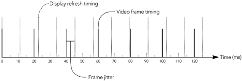
There are three possible occasions for adaptation to occur: (1) when the display device has a higher frame rate than the capture device, (2) when the display device has a lower frame rate than the capture device, and (3) when the display and capture devices run at the same nominal rate.
If the display device has a higher frame rate than the capture device, possible presentation times will surround the desired time, and each frame can be mapped to a unique display refresh interval. The simplest approach is to display frames at the refresh interval closest to their playout time. One can achieve better results by moving frames in the direction of any required playout adjustment: displaying a frame at the refresh interval following its playout time if the receiver clock is relatively fast, or at the earlier interval if the receiver clock is slow. Intermediate refresh intervals, when no new frames are received from the sender, can be filled by repetition of the previous frame.
If the display device has a lower frame rate than the capture device, displaying all frames is not possible, and the receiver must discard some data. For example, the receiver may calculate the difference between the frame playout time and the display times, and choose to display the subset of frames closest to possible display times.
If the display device and capture device run at the same rate, the playout buffer can be slipped so that frame presentation times align with the display refresh times, with the slippage providing some degree of jitter buffering delay. This is an uncommon case: Clock skew is common, and periodic jitter adjustments may upset the time-line. Depending on the direction of the required adjustment, the receiver must then either insert or remove a frame to compensate.
One can insert a frame into the playout sequence simply by repeating it for two intervals. Likewise, removing a frame from the sequence is a straightforward matter. (Note that other frames may be predicted from a nondisplayed frame, so it is often impossible to completely discard a frame without decoding, except for the last predicted frame before a full frame.)
No matter how the adjustment is made, note that the human visual system is somewhat sensitive to nonuniform playout, and the receiver should seek to keep the interframe presentation times as uniform as possible to prevent disturbing artifacts. Inserting or removing frames should be considered a last-resort operation, after smaller playout adjustments (choosing an earlier or later display frame time) have proven insufficient.
The final stages of the playout process are to decode the compressed media, mix media streams together if there are fewer output channels than active sources, and finally play the media to the user. This section considers each stage in turn.
For each active source the application must maintain an instantiation of the media decoder, comprising the decompression routines along with state known as the compression context. The decoder may be an actual hardware device or a software function, depending on the system. It converts each compressed frame into uncompressed media data, on the basis of the data in the frame and the compression context. As each frame is decoded, the compression context for the source is updated as shown in Figure 6.19.
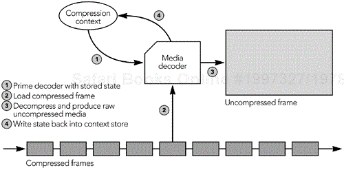
The presence of accurate state in the decompression context is fundamental to correct operation of the decoder, and codecs will produce incorrect results if the context is missing or damaged. This is most often an issue if some data packets are lost because there will be a frame that cannot be decoded. The result will be a gap in the playout where that frame should have been, but the decompression context will also be invalidated and the following frames will be corrupted.
Depending on the codec, it may be possible to feed it an indication that a frame has been lost, allowing the decoder to better repair the context and reduce the damage to the media stream (for example, many speech codecs have the notion of erasure frames to signal losses). Otherwise the receiver should try to repair the context and conceal the effects of the loss, as discussed in Chapter 8, Error Concealment. Many loss concealment algorithms operate on the uncompressed media data, after decoding and before mixing and playout operation.
Mixing is the process of combining multiple media streams into one, for output. This is primarily an issue for audio applications because most systems have only a single set of speakers but multiple active sources—for example, in a multiparty teleconference. Once audio streams have been decoded, they must be mixed together before being written to the audio device. The final stages of an audio tool will typically be structured somewhat as shown in Figure 6.20. The decoder produces uncompressed audio data on a per-source basis, written into a per-source playout buffer, and the mixer combines the results into a single buffer for playout (these steps can, of course, be combined into one if the decoder understands the mixing process). Mixing can occur at any time after the media has been decoded, and before it is due for playout.

The mix buffer is initially empty—that is, full of silence—and each participant's audio is mixed into the buffer in turn. The simplest approach to mixing is saturating addition, in which each participant's audio is added to the buffer in turn, with overflow conditions saturating at extreme values. In pseudocode, assuming 16-bit samples and mixing a new participant (src) into the buffer (mix_buffer), this becomes
audio_mix(sample *mix_buffer, sample *src, int len)
{
    int i, tmp;
    for(i = 0; i < len; i++) {
        tmp = mix_buffer[i] + src[i];
        if (tmp > 32767) {
            tmp = 32767;
        } else if (tmp < -32768) {
            tmp = -32768;
        }
        mix_buffer[i] = tmp;
    }
}
Other algorithms are possible if higher-fidelity mixing is required. Mixing samples is a task for which SIMD processors often have instructions. For instance, the Intel MMX (Multimedia Extensions) instructions include saturating-add instructions that add four 16-bit samples at a time, and because the mixing loop no longer has the branch checks, the performance can be up to ten times faster.
The actual mix buffer can be implemented as a circular buffer. The buffer is implemented as an array with start and end pointers, wrapping around to give the illusion of a continuous buffer (see Figure 6.21).

A limitation of the simple circular buffer is that it cannot always make a continuous buffer available for readout. Instead, as the readout nears the wrap-around point, it will be necessary to return two blocks of mixed data: one from the end of the circular buffer, one from the beginning. The need to return two buffers can be avoided if an array of twice the required size is allocated. If the readout routine requests a block that includes the wrap-around point in the circular buffer, the mixer can copy data into the additional space and return a pointer to a continuous block of memory as shown in Figure 6.22. This requires an additional copy of the audio data, up to half the size of the circular buffer, but allows the readout to return a single contiguous buffer, simplifying code that uses the mixer. Normal operation of the circular buffer is unchanged, except for a single copy when data is being read out.
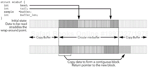
The process by which audio is played to the user is typically asynchronous, allowing the system to play one frame of audio while processing the next. This capability is essential to normal operation because it allows continuous playback even though the application is busy with RTP and media processing. It also shields the application from variations in the behavior of the system, perhaps due to other applications running on that system.
Asynchronous playout is especially important on general-purpose operating systems with limited support for multimedia applications. These systems are typically designed to give good average response, but often they have undesirable worst-case behavior, and typically they cannot guarantee that real-time applications are scheduled appropriately. An application can use asynchronous playout to its advantage, using the audio DMA (directory memory access) hardware to maintain continual playout.83 As shown in Figure 6.23, an application can monitor the occupancy of the output buffer and adjust the amount it writes to the audio device according to the time since it was last scheduled, such that the buffer occupancy after each iteration is constant.
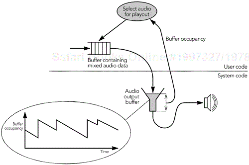
If the application detects a period of unusual scheduling latency—perhaps due to heavy disk activity on the system—it can preemptively increase the size of the audio DMA buffer, up to the limit imposed by the playout point. If the operating system does not allow direct monitoring of the amount of audio buffered and awaiting playout, it may be possible to derive an estimate from the amount of audio waiting to be read for the encoding side of the application. In many cases, audio playback and recording are driven from the same hardware clock, so an application can count the number of audio samples it records and use this information to derive the occupancy of the playback buffer. Careful monitoring of the audio DMA buffer can ensure continual playout in all but the most extreme environments.
Video playout is largely dictated by the refresh rate of the display, which determines the maximum time between the application writing to the output buffer and the image being presented to the user. The key to smooth video playout is twofold: (1) Frames should be presented at uniform rate, and (2) changes to a frame should be avoided while the video is being rendered. The first point is a matter for the playout buffer, selecting the appropriate display time as described in the section Playout Adaptation for Video earlier in this chapter.
The second point relates to the display: Frames are not presented instantaneously; instead they are drawn in a series of scan lines, left to right, top to bottom. This serial presentation allows the possibility that the application will be able to change a frame while it is being displayed, causing a glitch in the output. Double buffering can solve this problem, one buffer being used to compose a frame while the second buffer is being displayed. The two buffers are switched between frames, synchronized with the interframe gap. The means by which double buffering is achieved is system dependent but usually part of the video display API.
This chapter has described the fundamental behavior of RTP senders and receivers in some detail, focusing especially on the design of the receiver's playout buffer. The playout buffer design is relatively simple for streaming applications, which can accept several hundred milliseconds (or perhaps even seconds) of delay. For applications designed for interactive use, however, the play-out buffer is critical to achieving good performance. These applications need low latency, and hence playout buffer delays of a few tens of milliseconds, taxing the design of algorithms that must balance the needs of low delay with the need to avoid discarding late packets if possible.
RTP systems place a lot of intelligence in the end systems, leaving them to compensate for the variability inherent in a best-effort packet network. Recognizing this is the key to good performance: A well-designed, robust implementation can perform significantly better than a naive design.