Scientific and Mathematical Constants in SciPy

Before we begin, let’s complete the ritual of creating a new directory for this chapter. Please create a directory, chapter 11, for this chapter.

cd ∼
cd book
cd code
mkdir chapter11
cd chapter11

Now start the Jupyter Notebook App with the following command:

jupyter notebook

Open a new notebook and rename it to Chapter11_Practice. This notebook will hold the code for this chapter.

The SciPy library has a module called scipy.constants which has the values of many important mathematical and scientific constants. Let’s try a few of them. Run the following code in the notebook:

import numpy as np
import matplotlib.pyplot as plt
from scipy.constants import *
print("Pi = " + str(pi))
print("The golden ratio = " + str(golden))
print("The speed of light = " + str(c))
print("The Planck constant = " + str(h))
print("The standard acceleration of gravity = " + str(g))
print("The Universal constant of gravity = " + str(G))

The output is as follows:

Pi = 3.141592653589793
The golden ratio = 1.618033988749895
The speed of light = 299792458.0
The Planck constant = 6.62606957e-34,
The standard acceleration of gravity = 9.80665
The Universal constant of gravity = 6.67384e-11

Note that the SciPy constants do not include a unit of measurement, only the numeric value of the constants. These are very useful in numerical computing.

Linear algebra

Now we will study a few methods related to linear algebra. Let’s get started with the inverse of a matrix:

import numpy as np
from scipy import linalg
a = np.array([[1, 4], [9, 16]])
b = linalg.inv(a)
print(b)

The following is the output:

[[-0.8   0.2 ]
 [ 0.45 -0.05]]

We can also solve the matrix equation ax = b as follows:

a = np.array([[3, 2, 0], [1, -1, 0], [0, 5, 1]])
b = np.array([2, 4, -1])
from scipy import linalg
x = linalg.solve(a, b)
print(x)
print(np.dot(a, x))

The following is the output:

[ 2. -2.  9.]
[ 2.  4. -1.]

We can calculate the determinant of a matrix as follows:

a = np.array([[0, 1, 2], [3, 4, 5], [6, 7, 8]])
print(linalg.det(a))

Run the code above in the notebook and see the results for yourself.

We can also calculate the norms of a matrix as follows:

a = np.arange(16).reshape((4, 4))
print(linalg.norm(a))
print(linalg.norm(a, np.inf))
print(linalg.norm(a, 1))
print(linalg.norm(a, -1))

The following are the results:

35.2136337233
54
36
24

We can also compute QR and RQ decompositions as follows:

from numpy import random
from scipy import linalg
a = random.randn(3, 3)
q, r = linalg.qr(a)
print(a)
print(q)
print(r)
r, q = linalg.rq(a)
print(r)
print(q)

Integration

SciPy has the integrate module for various integration operations, so let’s look at a few of its methods. The first one is quad(). It accepts the function to be integrated as well as the limits of integration as arguments, and then returns the value and approximate error. The following are a few examples:

from scipy import integrate
f1 = lambda x: x**4
print(integrate.quad(f1, 0, 3))
import numpy as np
f2 = lambda x: np.exp(-x)
print(integrate.quad(f2, 0, np.inf))

The following are the outputs:

(48.599999999999994, 5.39568389967826e-13)
(1.0000000000000002, 5.842606742906004e-11)

trapz() integrates along a given axis using the trapezoidal rule:

print(integrate.trapz([1, 2, 3, 4, 5]))

The following is the output:

12.0

Let’s see an example of cumulative integration using the trapezoidal rule.

import matplotlib.pyplot as plt
x = np.linspace(-2, 2, num=30)
y = x
y_int = integrate.cumtrapz(y, x, initial=0)
plt.plot(x, y_int, 'ro', x, y[0] + 0.5 * x**2, 'b-')
plt.show()

The following (Figure 11-1) is the output:

Figure 11-1. Cumulative integration using the trapezoidal rule

Interpolation

This module has methods for interpolation. Let’s study a few of these with the help of the graphical representation of matplotlib. interp1d() is used for 1-D interpolation as demonstrated below.

from scipy import interpolate
x = np.arange(0, 15)
y = np.exp(x/3.0)
f = interpolate.interp1d(x, y)
xnew = np.arange(0, 14, 0.1)
ynew = f(xnew)
plt.plot(x, y, 'o', xnew, ynew, '-')
plt.show()

The following (Figure 11-2) is the result:

Figure 11-2. 1-D interpolation

interp1d() works for y=f(x) type of functions. Simillary, interp2d() works on z=f(x, y) type of functions. It is used for two-dimensional interpolation.

x = np.arange(-5.01, 5.01, 0.25)
y = np.arange(-5.01, 5.01, 0.25)
xx, yy = np.meshgrid(x, y)
z = np.sin(xx**3 + yy**3)
f = interpolate.interp2d(x, y, z, kind='cubic')
xnew = np.arange(-5.01, 5.01, 1e-2)
ynew = np.arange(-5.01, 5.01, 1e-2)
znew = f(xnew, ynew)
plt.plot(x, z[0, :], 'ro-', xnew, znew[0, :], 'b-')
plt.show()

The following (Figure 11-3) is the result:

Figure 11-3. 2-D interpolation

Next, we are going to study splev(), splprep(), and splrep(). The splev() method is used to evaluate B-spline or its derivatives. We will use this method along with splprep() and splrep(), which are used for representations of B-spline.

splrep() is used for representation of a 1-D curve as follows:

from scipy.interpolate import splev, splrep
x = np.linspace(-10, 10, 50)
y = np.sinh(x)
spl = splrep(x, y)
x2 = np.linspace(-10, 10, 50)
y2 = splev(x2, spl)
plt.plot(x, y, 'o', x2, y2)
plt.show()

The following (Figure 11-4) is the result:

Figure 11-4. Representation of a 1-D curve

splprep() is used for representation of an N-dimensional curve.

from scipy.interpolate import splprep
theta = np.linspace(0, 2*np.pi, 80)
r = 0.5 + np.cosh(theta)
x = r * np.cos(theta)
y = r * np.sin(theta)
tck, u = splprep([x, y], s=0)
new_points = splev(u, tck)
plt.plot(x, y, 'ro')
plt.plot(new_points[0], new_points[1], 'r-')
plt.show()                                                                                                                                                

The following (Figure 11-5) is the result.

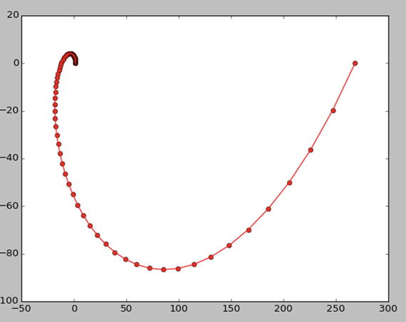
Figure 11-5. Representation of an N-D curve

Conclusion

In this chapter, we were introduced to a few important and frequently used modules in the SciPy library. The next two chapters will be focused on introducing readers to the specialized scientific areas of signal and image processing. In the next chapter, we will study a few modules related to the area of signal processing.