Waveforms

Let’s get started with the waveform generator functions. Create a new directory chapter 12 in the ∼/book/code directory. Run the following command to start the Jupyter Notebook App:

jupyter notebook

Rename the current notebook to Chapter12_Practice. As in previous chapters, run all the code from this chapter in the same notebook. Let’s import NumPy and matplotlib first.

import numpy as np
import matplotlib.pyplot as plt

The first example we will study is a sawtooth generator function.

from scipy import signal
t = np.linspace(0, 2, 5000)
plt.plot(t, signal.sawtooth(2 * np.pi * 4 * t))
plt.show()

The function accepts the time sequence and the width of signal and generates triangular or sawtooth shaped continuous signals. The following (Figure 12-1) is the output,

Figure 12-1. Sawtooth wave signal

Let’s have a look at a square wave generator which accepts time array and duty cycle as inputs.

t = np.linspace(0, 1, 400)
plt.plot(t, signal.square(2 * np.pi * 4 * t))
plt.ylim(-2, 2)
plt.title('Square Wave')
plt.show()

The output is as follows:

Figure 12-2. Square wave signal

A pulse-width modulated square sine wave can be demonstrated as follows:

sig = np.sin(2 * np.pi * t)
pwm = signal.square(2 * np.pi * 30 * t, duty=(sig +1)/2)
plt.subplot(2, 1, 1)
plt.plot(t, sig)
plt.title('Sine Wave')
plt.subplot(2, 1, 2)
plt.plot(t, pwm)
plt.title('PWM')
plt.ylim(-1.5, 1.5)
plt.show()

The output (Figure 12-3) is as follows:

Figure 12-3. Modulated wave

Window Functions

A window function is a mathematical function which is zero outside a specific interval. We will now look at three different window functions. The first one is the Hamming window function. We have to pass the number of points in the output window as an argument to all the functions.

window = signal.hamming(101)
plt.plot(window)
plt.title('Hamming Window Function')
plt.xlabel('Sample')
plt.ylabel('Amplitude')
plt.show()

The output (Figure 12-4) is as follows:

Figure 12-4. Hamming window demo

The Hanning window function is as follows:

window = signal.hanning(101)
plt.plot(window)
plt.title('Hanning Window Function')
plt.xlabel('Sample')
plt.ylabel('Amplitude')
plt.show()

The output (Figure 12-5) is as follows:

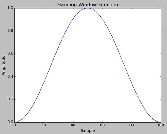
Figure 12-5. Hanning window demo

The Kaiser window function is as follows,

window = signal.kaiser(51, beta=20)
plt.plot(window)
plt.title('Kaiser Window Function Beta = 20')
plt.xlabel('Sample')
plt.ylabel('Amplitude')
plt.show()                                                                                                                                                

The output (Figure 12-6) is as follows:

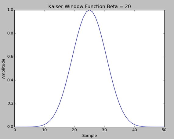
Figure 12-6. Kaiser window demo

Mexican Hat Wavelet

We can generate a Mexican hat wavelet with the Ricker function by passing the number of points and the amplitude as parameters, as in the following:

plt.plot(signal.ricker(200, 6.0))
plt.show()

The Mexican hat wavelet is a special case in the family of continuous wavelets. It is used for filtering and averaging spectral signals. The output is as follows:

Figure 12-7. Mexican hat wavelet

Convolution

We can convolve two N-dimensional arrays with the convolve() method as follows:

sig = np.repeat([0., 1., 0.], 100)
win = signal.hann(50)
filtered = signal.convolve(sig, win, mode='same') / sum(win)
plt.subplot(3, 1, 1)
plt.plot(sig)
plt.ylim(-0.2, 1.2)
plt.title('Original Pulse')
plt.subplot(3, 1, 2)
plt.plot(win)
plt.ylim(-0.2, 1.2)
plt.title('Filter Impulse Response')
plt.subplot(3, 1, 3)
plt.plot(filtered)
plt.ylim(-0.2, 1.2)
plt.title('Filtered Signal')
plt.show()

The signal, the window, and the convolution of those are as shown in Figure 12-8. Convolution of two signals provides a combination of both the signals to form a third signal. It is a very important signal combination technique in signal processing. If the signals represent image or audio data, we get an improved image or audio based on the degree of convolution. If you have not noticed already, we are using the repeat() method of NumPy, which takes the pattern to be repeated and the number of repetitions as arguments. In this example, we’re generating a signal with the sample size of 300.

Figure 12-8. Convolution

Conclusion

In this short chapter, we were introduced to a few important classes of methods in the scipy.signal module of SciPy. In the next chapter, we will explore the area of image processing.