Basics of NumPy

NumPy is short for Numeric(al) Python . Its website ( http://www.numpy.org ) says:

NumPy is the fundamental package for scientific computing with Python

Its features are as follows:

It has a powerful custom N-dimensional array object for efficient and convenient representation of data.

It has tools for integration with other programming languages used for scientific programming like C/C++ and FORTRAN.

It is used for mathematical operations like linear algebra, matrix operations, image processing, and signal processing.

sudo pip3 install --upgrade pip
sudo pip3 install jupyter

Jupyter Notebooks

Jupyter notebooks are documents produced by the Jupyter Notebook App, which have Python code and Rich Text elements like paragraphs, equations, figures, links, and interactive visualizations. Notebooks have human-readable components and machine-readable (executable) components.

Let’s get started with NumPy and Jupyter notebooks now. Open lxterminal and run the following sequence of commands :

cd ∼
cd book
cd code
mkdir chapter10
cd chapter10

This will create and navigate to the directory corresponding to the current chapter, chapter10.

Now, this is our notebook startup folder, so let’s launch the notebook from here with the following command:

jupyter notebook

It will start the Jupyter Notebook App and a browser window (Chromium browser in the latest releases of Raspbian) will open.

The following (Figure 10-1) is a screenshot of the console when the Jupyter notebook starts:

Figure 10-1. Jupyter Notebook App console

The following (Figure 10-2) is a screenshot of the Chromium browser window tab running the notebook app:

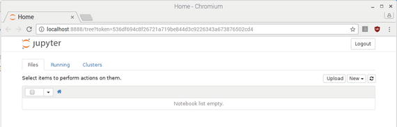
Figure 10-2. Jupyter Notebook App running in Chromium

In the upper right part of the browser window click New and then in the subsequent dropdown select Python 3. See the following (Figure 10-3) screenshot:

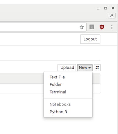
Figure 10-3. New Python 3 notebook

It will open a new notebook tab (Figure 10-4) in the same browser window.

Figure 10-4. Python 3 notebook tab

Change the name of the Jupyter notebook to Chapter10_Practice as shown in the screenshot (Figure 10-5) below.

Figure 10-5. Renaming the notebook

The Notebook app will show an instance of a new notebook with the updated name, with status as “running,” as shown in the screenshot (Figure 10-6) below.

Figure 10-6. Notebook running

Now, if you check the Chapter10 directory, you will find a file Chapter10_Practice.ipynb corresponding to the notebook.

In the menubar at the top of the window, there are options like you would have in any other IDE—for example, save, copy, paste, and run.

Type import numpy as np in the first cell and click the Run button. The control will automatically create the next text cell and focus the cursor on it as shown below (Figure 10-7).

Figure 10-7. Working with Python 3 code

We have just imported NumPy to our notebook, so we do not have to import again. Also, we can edit the previous cells of the notebook too. At the type of execution, if the interpreter highlights a mistake in the syntax, we can fix it by editing any of the cells. We will learn more about Jupyter as we go forward in scientific computing.

x = np.array([1, 2, 3], np.int16)
y = np.array([[0, 1, 2], [3, 4, 5]], np.int32)
z = np.array([[[0, 1, 2], [2, 3, 4], [4, 5, 6]],[[1, 1, 1], [0, 0, 0], [1, 1, 1]]], np.float16)

print(x.shape)
print(y.shape)
print(z.shape)

(3,)
(2, 3)
(3, 3, 3)

print(z[:,1])

[[ 2.  3.  4.]
 [ 0.  0.  0.]]

print(z.shape)
print(z.ndim)
print(z.size)
print(z.itemsize)
print(z.nbytes)
print(z.dtype)

(2, 3, 3)
3
18
2
36
float16

Array Creation Routines

Let’s create ndarrays with built-array creation routines . We are also going to use matplotlib to visualize the arrays created. We will use matplotlib for visualizing the data as and when needed. The last chapter of this book is dedicated to matplotlib, where we will learn more about it.

The first method for creating ndarrays is ones(). As you must have guessed, it creates arrays where all the values are ones. Run the following statements in the notebook to see a demonstration of the method:

a = np.ones(5)
print(a)
b = np.ones((3,3))
print(b)
c = np.ones((5, 5), dtype=np.int16)
print(c)

Similarly we have the np.zeros() method for generating multidimensional arrays of zeros. Just run the examples above by passing the same set of arguments to the method np.zeros(). The np.eye() method is used for creating diagonal matrices. We can also specify the index of the diagonals. Run the following examples in the notebook for a demonstration:

a = np.eye(5, dtype=np.int16)
print(a)
b = np.eye(5, k=1)
print(b)
c = np.eye(5, k=-1)
print(c)

np.arange() returns a list of evenly spaced numbers in a specified range. Try the following examples in the notebook:

a = np.arange(5)
print(a)
b = np.arange(3, 25, 2)
print(b)

The output is as follows:

[0 1 2 3 4]
[ 3  5  7  9 11 13 15 17 19 21 23]

Let’s have some fun with matplotlib now. Run the following example in the notebook:

import matplotlib.pyplot as plt
x = np.arange(10)
y = np.arange(10)
print(x)
print(y)
plt.plot(x, y, 'o')
plt.show()

In the example above, we are graphically representing the ndarrays. The text result is as follows:

[0 1 2 3 4 5 6 7 8 9]
[0 1 2 3 4 5 6 7 8 9]

The graphical output (Figure 10-8) is as follows:

Figure 10-8. Graphical Output of arange()

With the statement import matplotlib.pyplot as plt, we are importing the pyplot module of the myplotlib library. plt.plot() prepares the plot graph for display and plt.show() displays it on the screen.

We have a similar method, np.linspace(), for generating a linear array. The major difference between linspace() and arange() is that linspace() accepts the number of samples to be generated as an argument rather than stepsize. The following code snippet shows the way linspace() generates the data:

N = 8
y = np.zeros(N)
x1 = np.linspace(0, 10, N)
x2 = np.linspace(0, 10, N)
plt.plot(x1, y - 0.5, 'o')
plt.plot(x2, y + 0.5, 'o')
plt.ylim([-1, 1])
plt.show()

plt.ylim() specifies the limit of the Y co-ordinate on the graph. The following (Figure 10-9) is the output:

Figure 10-9. linspace() graph

Similarly, we have the logspace() method which generates the array value on a logarithmic scale. The following code demonstrates that:

N = 64
x = np.linspace(1, N, N)
y = np.logspace(0.1, 1, N)
plt.plot(x, y, 'o')
plt.show()

Run the statements in the notebook and it generates the following (Figure 10-10) output:

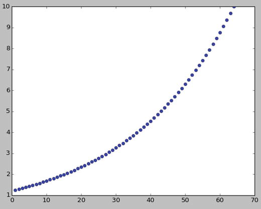
Figure 10-10. linspace() versus logspace() graph

Matrix and Linear Algebra

NumPy has routines for matrix creation. Let’s see a few examples. np.matrix() interprets the given data as a matrix. The following are examples:

a = np.matrix('1 2; 3 4')
b = np.matrix([[1, 2], [3, 4]])
print(a)
print(b)

Run the code in the notebook and you will see that both the examples return the matrices even though the input was in a different format.

[[1 2]
 [3 4]]
[[1 2]
 [3 4]]

np.bmat() builds a matrix from arrays or sequences.

A = np.mat('1 1; 1 1')
B = np.mat('2 2; 2 2')
C = np.mat('3 4; 5 6')
D = np.mat('7 8; 9 0')
a = np.bmat([[A, B], [C, D]])
print(a)

The code above returns a matrix combined from all the sequences. Run the code in the notebook to see the output as follows:

[[1 1 2 2]
 [1 1 2 2]
 [3 4 7 8]
 [5 6 9 0]]

np.matlib.zeros() and np.matlib.ones() return the matrices of zeros and ones respectively. np.matlib.eye() returns a diagonal matrix. np.matlib.identity() returns a square identity matrix of a given size. The following code example demonstrates these methods:

from numpy.matlib import *
a = zeros((3, 3))
print(a)
b = ones((3, 3))
print(b)
c = eye(3)
print(c)
d = eye(5, k=1)
print(d)
e = eye(5, k=-1)
print(e)
f = identity(4)
print(f)

The rand() and randn() methods return matrices with random numbers.

a = rand((3, 3))
b = randn((4, 4))
print(a)
print(b)

Let’s study a few methods related to linear algebra (matrix operations). We have the dot() method, which calculates the dot product of two arrays, whereas vdot() calculates the dot product of two vectors. inner() calculates the inner product of two arrays. outer() calculates the outer product of two vectors. The following code example demonstrates all these methods:

a = [[1, 0], [0, 1]]
b = [[4, 1], [2, 2]]
print(np.dot(a, b))
print(np.vdot(a, b))
print(np.inner(a, b))
print(np.outer(a, b))

The output is as follows:

[[4 1]
 [2 2]]
6
[[4 2]
 [1 2]]
[[4 1 2 2]
 [0 0 0 0]
 [0 0 0 0]
 [4 1 2 2]]

Trigonometric Methods

Let’s visualize trigonometric methods. We will visualize sin(), cos(), tan(), sinh(), and cosh() methods with matplotlib. The following example demonstrates the usage of these methods:

x = np.linspace(-np.pi, np.pi, 201)
plt.plot(x, np.sin(x))
plt.xlabel('Angle in radians')
plt.ylabel('sin(x)')
plt.show()

The output (Figure 10-11) is as follows:

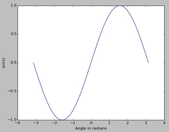
Figure 10-11. Graph for sin(x)

The following code examples demonstrate usage of cos():

x = np.linspace(-np.pi, 2*np.pi, 401)
plt.plot(x, np.cos(x))
plt.xlabel('Angle in radians')
plt.ylabel('cos(x)')
plt.show()

The following (Figure 10-12) is the output:

Figure 10-12. graph for cos(x)

Let’s move on to the hyperbolic Cosine and Sine waves as follows,

x = np.linspace(-5, 5, 2000)
plt.plot(x, np.cosh(x))
plt.show()
plt.plot(x, np.sinh(x))
plt.show()

The following (Figure 10-13) is the output of cosh():

Figure 10-13. Graph of cosh(x)

The following (Figure 10-14) is the graph of sinh(x):

Figure 10-14. Graph of sinh(x)

Random Numbers and Statistics

The rand() method generates a random matrix of given dimensions. The randn() method generates a matrix with numbers sampled from the normal distribution. randint() generates a number in given limits excluding the limits. random_integers() generates a random integer including the given limits. The following code demonstrates the first three of the above methods:

import numpy as np
a = np.random.rand(3, 3)
b = np.random.randn(3, 3)
c = np.random.randint(4, 15)
print(a)
print(b)
print(c)

We can calculate median, average, mean, standard deviation, and variance of a ndarray as follows:

a = np.array([[10, 7, 4], [1, 2, 3], [1, 1, 1]])
print(median(a))
print(average(a))
print(mean(a))
print(std(a))
print(var(a))

Fourier Transforms

NumPy has a module for basic signal processing. The fft module has the fft() method, which is used for computing one-dimensional discrete Fourier transforms as follows:

t = np.arange(256)
sp = np.fft.fft(np.sin(t))
freq = np.fft.fftfreq(t.shape[-1])
plt.plot(freq, sp.real, freq, sp.imag)
plt.show()

The output (Figure 10-15) is as follows:

Figure 10-15. Fast Fourier Transform

fft2() and fftn() are used for calculating two-dimensional and n-dimensional discrete Fourier transforms respectively. Try to write code for these.

Conclusion

In this chapter, we got started with NumPy, matplotlib, and Jupyter, and we learned how to perform numeric computations and basic visualizations in Python. In the next chapter, we will get started with the SciPy Library.