
Chapter 11
Nonlinear Projections

Clouds image courtesy of Phillipe Hurbain
Objectives
By the end of this chapter, you should:
- understand how angular fisheye projection works;
- have implemented a fisheye camera;
- understand how spherical panoramic projection works;
- have implemented a spherical panoramic camera;
- have the tools to produce interesting images using nonlinear projections.
This chapter highlights one of the many advantages that ray tracing has over other graphics algorithms: it’s simple to implement projections that are different from the orthographic and perspective projections discussed in previous chapters. In these projections, the field of view is determined by shooting rays from the eye point through points on the view plane. They are known as linear projections because the projectors are straight lines.
There are, however, an infinite number of other ways that we can define ray directions at the eye point from sample points on the view plane. These are nonlinear projections in which the rays do not go through the view-plane sample points. Provided we can define the ray directions, we can implement a camera based on them.
I’ll present here two nonlinear projections: a fisheye projection and a spherical panoramic projection. These both allow us to render the whole scene that surrounds the eye point, a feat that’s not possible with perspective or orthographic projections. The resulting images can be surreal and wonderful. But these projections also have important practical applications. For example, fisheye projections are used in planetariums and other immersive viewing environments (see the Further Reading section). Another projection technique that’s used for immersive environments is a cylindrical panoramic projection, but I’ve left that as an exercise. Most of the applications of these projections involve real-time animated immersive displays, for which the images in this chapter can’t do justice. This chapter will, however, give you an understanding of how two types of nonlinear projections are implemented in ray tracing.
11.1 Fisheye Projection
11.1.1 Theory
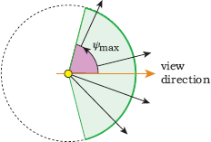
A fisheye projection uses a view volume that’s an infinite circular cone with apex at the eye point and centered on the view direction. Figure 11.1 shows a cross section of part of a view volume that’s inside a unit sphere centered on the eye point. The half angle of the cone ψmax ∊ [0, 180°] defines the field of view (fov), where the value ψmax = 180° provides the full 360° field of view around the eye point.1 Within the cone, rays can be shot in any direction. In other words, we can regard the rays as being shot through the surface of a sphere.
For comparison, Figure 11.2 shows a perspective projection in cross section where the field of view is determined by the size of the window and its distance from the eye point. Rays are shot through the window.

In perspective projection, the field of view is determined by the window size and its distance from the eye point.
A fisheye projection differs from this in two ways. First, only pixels in a circular disk centered on the window have rays associated with them. Second, the field of view is independent of the location and size of the window.
Figure 11.3(a) shows a cross section of a fisheye projection and a window. For a given point on the window, we compute the angle ψ that its ray makes with the viewing direction. This will only be a function of the straight-line distance r between the point and the center of the window. As a result, concentric circles around the center of the window map to constant values of ψ (see Figure 11.3(b)). The value ψ is 0 in the middle of the window, and the edge of the disk is mapped to ψmax. We therefore only render square images and only trace rays for pixels in the disk, but see Exercise 11.10. The viewing geometry is rotationally symmetric about the view direction. The key point here is that the ray directions are not constrained by the straight-line geometry that connects the eye and pixel points in linear projections; instead, rays are only associated with pixel points by a mathematical expression that we devise.
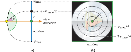
(a) In a fisheye projection, the field of view is independent of the size of the window and its distance from the eye point; (b) only pixels in a disk centered on the window have rays traced.
Although we can specify how ψ varies with r any way we want to, the fisheye projection I’ll discuss here has ψ proportional to r, as this is the simplest technique (see Equation (11.3)). Figure 11.4 shows two special cases of this fisheye projection in cross section. Figure 11.4(a) shows a 180° (ψmax = 90°) projection, while Figure 11.4(b) shows a 360° (ψmax = 180°) projection. The dashed lines simply associate points on the window with ray directions; their shapes don’t mean anything.

Schematic relationship between points on the view-plane window and fisheye-camera ray directions: (a) 180° view; (b) 360° view.
For each sample point on the view plane, we perform the following tasks:
- compute the distance r;
- if the pixel is inside the disk, compute ψ(r);
- compute the ray direction in world coordinates.
To carry out these tasks, we first transform the view-plane coordinates of a sample point (xp, yp) ∊ [−shres / 2, −svres / 2] × [shres/2, svres / 2] to normalized device coordinates, (xn, yn) ∊ [−1, +1] × [−1, +1].2 (see Figure 11.5). I’ve drawn Figure 11.5(a) with hres ≠ vres, because a variation of the fisheye projection allows us to render rectangular images, and so does spherical panoramic projection. Both projection techniques use the transformation to normalized device coordinates. The transformation equations are
xn=2shresxp,yn=2svresyp. (11.1)

See Exercise 11.1. We next check that the square of the distance from the origin satisfies
r2=x2n+y2n≤1.0, (11.2)
and if this is satisfied, we compute ψ with
ψ(r)=rψmax. (11.3)
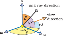
To compute the ray direction in world coordinates, we use Equations (11.1) and (11.3), with the orthonormal basis of the fisheye camera. Although the (u, v, w) vectors have the same orientation as a pinhole camera, the calculation of the ray direction is quite different. This is because we don’t have the coordinates (xp, yp, −d) to work with as in perspective projection; instead, we have to work with angles. The angles are also different from the standard spherical coordinate angles discussed in Chapter 2. For example, ψ is measured from the view direction (−w).
I’ve illustrated how to compute the ray direction d with three 2D diagrams in Figure 11.6. I’ve also made the ray direction a unit vector from the start to simplify the calculations. This places the vector ends on a unit sphere centered on the eye point. Figure 11.6(a) shows the projections of the ray onto the view direction and the (u, v) plane. This figure is drawn from an arbitrary point on the (u, v) plane. The projected length of the vector in the viewing direction is cos ψ, and on the (u, v) plane is sin ψ.

(a) A unit ray direction d projected onto the view direction (orange arrow) and onto the (u, v) plane (the vertical cyan line); (b) the (xn, yn)-coordinates determine the angle α that r makes with the u-direction when it’s projected onto the (u, v)-plane; (c) the projections of d onto the u- and v-directions.
Figure 11.6(b) shows the normalized device coordinates and the angle α that the line r makes with the xn-axis. Fortunately, we only need the sine and cosine of α:
sinα=yn/r,cosα=xn/r.
Figure 11.6(c) shows the projections of d onto the (u, v) plane, where from Figure 11.6(a), the vector’s length is foreshortened to sin ψ. We can now write the expression for d:
d=sinψcosα u+sinψsinα v-cos ψ w. (11.4)
Note that this is a unit vector by construction (see Exercise 11.7).
11.1.2 Implementation
The fisheye projection is implemented with a Fisheye camera, whose class declaration appears in Listing 11.1. The only new data member is psi_max.
The FishEye::render_scene function appears in Listing 11.2.
class Fisheye: public Camera {
public:
// constructors, etc.
Vector3D
ray_direction(const Point2D& p, const int hres,
const int vres, const float s, float& r) const;
virtual void
render_scene(World& w);
private:
float psi_max; // in degrees
};
Listing 11.1. Declaration of the camera class FishEye.
void
FishEye::render_scene(World& wr) {
RGBColor L;
ViewPlane vp(wr.vp);
int hres = vp.hres;
int vres = vp.vres;
float s = vp.s;
Ray ray;
int depth = 0;
Point2D sp; // sample point in [0, 1] X [0, 1]
Point2D pp; // sample point on the pixel
float r_squared; // sum of squares of normalized device
coordinates
wr.open_window(vp.hres, vp.vres);
ray.o = eye;
for (int r = 0; r < vres; r++) // up
for (int c = 0; c < hres; c++) { // across
L = black;
for (int j = 0; j < vp.num_samples; j++) {
sp = vp.sampler_ptr->sample_unit_square();
pp.x = s * (c - 0.5 * hres + sp.x);
pp.y = s * (r - 0.5 * vres + sp.y);
ray.d = ray_direction(pp, hres, vres, s, r_squared);
if (r_squared <= 1.0)
L += wr.tracer_ptr->trace_ray(ray, depth);
}
L /= vp.num_samples;
L *= exposure_time;
wr.display_pixel(r, c, L);
}
}
Listing 11.2. The function FishEye::render_scene.
The function ray_direction in Listing 11.3 computes the ray direction according to the theory presented in Section 11.1.1. Note that this function also returns the square of the normalized device coordinates and that the render_scene function only traces the ray when Equation (11.2) is satisfied.
The user interface of the fisheye camera doesn’t specify ψmax directly but instead allows users to specify a field of view = 2ψmax. This is more intuitive because, for example, if we want to render a 360° view, we can specify the field of view as 360° in the build function.
Vector3D
FishEye::ray_direction( const Point2D& pp, const int hres, const int
vres, const float s, float& r_squared) const {
// compute the normalized device coordinates
Point2D pn(2.0 / (s * hres) * pp.x, 2.0 / (s * vres) * pp.y);
r_squared = pn.x * pn.x + pn.y * pn.y;
if (r_squared <= 1.0) {
float r = sqrt(r_squared);
float psi = r * psi_max * PI_ON_180;
float sin_psi = sin(psi);
float cos_psi = cos(psi);
float sin_alpha = pn.y / r;
float cos_alpha = pn.x / r;
Vector3D dir = sin_psi * cos_alpha * u + sin_psi
* sin_alpha * v - cos_psi * w;
return (dir);
}
else
return (Vector3D(0.0));
}
Listing 11.3. The function FishEye::ray_direction.
11.1.3 Results
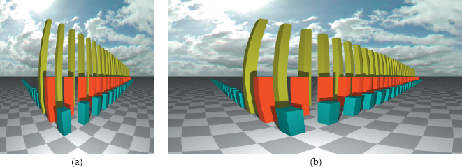
Now we can have some fun. Figure 11.7(a) shows a perspective view of the boxes from Chapter 9 with the green boxes increased in height, and a sky-dome with clouds.3 The scene is rendered with a pinhole camera looking horizontally.

Various views of rectangular boxes, a checker plane, and clouds rendered with a pinhole camera (a) and a fisheye camera in (b)–(e). The fisheye camera uses the following values for the fov: (b) 120°; (c) 180°; (d) 360°; (e) 360°; (f) 180°.
Figure 11.7(b)–(d) show the scene rendered with a fisheye camera that has the same eye and look-at points as the pinhole camera. The angle ψmax ranges from 60° in Figure 11.7(b) to 180° in Figure 11.7(d), which is the 360° view. An obvious fact from these images is that the fisheye projection doesn’t preserve straight lines, although some of the lines are straight (see Question 11.3).
Figure 11.7(e) shows another 360° view, this time with the camera looking in a downwards direction. Finally, Figure 11.7(f) shows the sky with the camera looking vertically up, ψmax = 90°, and no boxes. Real cameras with circular fisheye lenses can take photographs like this.
Figure 11.8 shows three views of the Uffizi Gallery buildings in Florence, Italy. Here, the only object in the scene is the cloud sphere in Figure 11.7 with the clouds replaced by the Uffizi image. This is based on one of Paul Debevec’s high dynamic light probe images at http://www.debevec.org/Probes, with a light probe mapping to render the scene. The camera is near the center of the sphere. I’ll discuss the light probe mapping in Chapter 29.
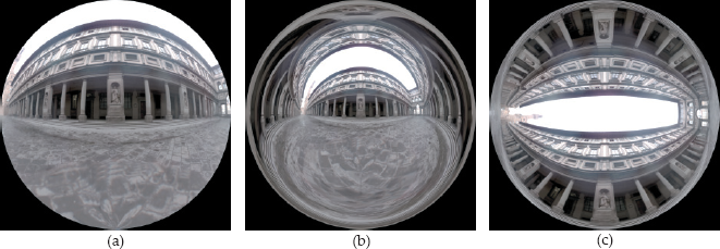
Three views of the Uffizi Gallery buildings: (a) fov = 180°; (b) fov = 360°; (c) looking up, fov = 100°. The Ufiizi Gallery image is courtesy of Paul Debevec.
As an example of how fisheye projections can be used for scientific visualization, Figure 11.9 shows photographs of an immersive dome that uses fisheye projections. This is in the Western Austalian Supercomputer Program (WASP) at the University of Western Australia.
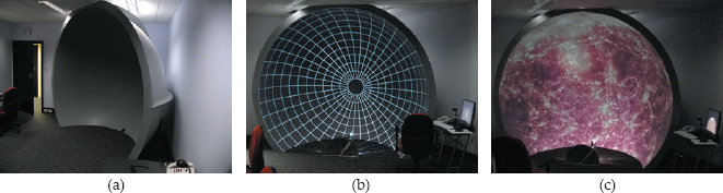
Immersive dome: (a) angle view; (b) grid test image; (c) cosmological simulation by Paul Burke. These images are from the website http://local.wasp.uwa.edu.au/~pbourke/exhibition/domeinstall/. Photographs courtesy of Paul Burke.
11.2 Spherical Panoramic Projection
11.2.1 Theory
A spherical panoramic projection is similar to a fisheye projection, but it has one major difference. We use the normalized device coordinates of a pixel point to define separate angles λ in the azimuth direction and ψ in the polar direction instead of a single radial angle. Figure 11.9 illustrates these angles, which are used to define the primary ray directions. The angle λ is in the (u, w) plane, and is measured counterclockwise from the view direction. The angle ψ is measured up from the (u, w) plane in a vertical plane. As such, λ and ψ have a simple relationship with the standard spherical coordinate angles θ and φ, also shown in Figure 11.10. The expressions are
φ=π-λ,θ=π/2-ψ. (11.5)
The angles λ and ψ and their relation to the standard spherical coordinate angles φ and θ.
We define ψ and λ as linear functions of the normalized device coordinates xn and yn as follows:
λ=xnλmax,ψ=ynψmax.
These result in (λ, ψ) ∊ [−λmax, λmax] × [−ψmax, ψmax], where λmax = 180° and ψmax = 90° give the full 360° × 180° field of view. The general fov is defined as 2λmax × 2ψmax .
By relating λ and ψ to the standard spherical coordinate angles in Equation (11.5), we can use Equations (2.3) with r = 1 to write the ray direction as
d=sinθsinφ u+cosθ v+sinθcosφ w. (11.6)
This is a unit vector by construction.
11.2.2 Implementation
The camera class that implements the spherical panoramic projection is just called Spherical. Listing 11.4 shows the implementation of the function Spherical::ray_direction. I won’t reproduce the spherical camera’s render_ scene function here, as the only difference between it and the fisheye’s function is the absence of the r2 factor.
The user interface of the Spherical camera allows the user to specify the horizontal and vertical fov angles separately.
11.2.3 Results
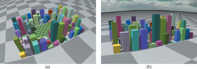
Images rendered with a spherical camera must have their aspect ratio equal to λmax/ψmax, otherwise the images will be distorted. Figure 11.11(a) shows a city modeled with random axis-aligned boxes and rendered with an fov of 84° × 56° at a pixel resolution of 600 × 400. Figure 11.11(b) is rendered with a view that shows the horizon.
Vector3D
Spherical::ray_direction( const Point2D& pp,
const int hres,
const int vres,
const float s ) const {
// compute the normalized device coordinates
Point2D pn( 2.0 / (s * hres) * pp.x, 2.0 / (s * vres) * pp.y);
// compute the angles lambda and phi in radians
float lambda = pn.x * lambda_max * PI_ON_180;
float psi = pn.y * psi_max * PI_ON_180;
// compute the spherical azimuth and polar angles
float phi = PI - lambda;
float theta = 0.5 * PI - psi;
float sin_phi = sin(phi);
float cos_phi = cos(phi);
float sin_theta = sin(theta);
float cos_theta = cos(theta);
Vector3D dir = sin_theta * sin_phi * u + cos_theta* v
+ sin_theta * cos_phi * w;
return (dir);
}
Listing 11.4. The function Spherical::ray_direction.
Figure 11.12 shows two views of the city with the camera above the central park and looking horizontally. Note that in these images, the vertical building edges are vertical straight lines, and the horizon is horizontal. This is a property of spherical projection images, but only when the camera looks horizontally. You should compare these images with Figure 11.11. In Figure 11.12(a), the fov = 180° × 120°. Figure 11.12(b) is rendered with the full view in each direction, fov = 360° × 180°. Such images must be rendered with an aspect ratio of 2.0.
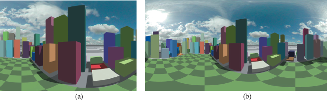
Figure 11.13 shows the Uffizi buildings rendered with fov = 360° × 180°.
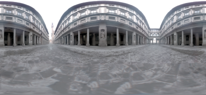
Full 360° × 180° spherical projection view of the Uffizi Gallery buildings with the view direction horizontal. The Uffizi Gallery image is courtesy of Paul Debevec.
Further Reading
The best place to read about the material in this chapter is Paul Burke’s wonderful website at http://local.wasp.uwa.edu.au/~pbourke/. Section 11.1.1 is based on material in http://local.wasp.uwa.edu.au/~pbourke/projection/fisheye/. This website also discusses different types of projections. The website http://local.wasp.uwa.edu.au/~pbourke/exhibition/domeinstall/ has photographs of numerous spherical dome installations that use fisheye projections. The website http://www.icinema.unsw.edu.au/projects/infra_avie.html has information about a state-of-the-art immersive visualization system that uses cylindrical panoramic projection.
Paul Debevec’s website at http://www.debevec.org/ and the links on this site have a large amount of information on high dynamic range imagery and light probes. The clouds image can be found on Phillipe Hurbain’s website at http://www.philohome.com/skycollec.htm.
Questions
- 11.1. Can you have a 180° field of view with perspective projection? If you could, would it be useful?
- 11.2. How do you zoom with the fisheye camera?
- 11.3. Which straight lines are preserved in fisheye projections?
- 11.4. How do you zoom with the spherical panoramic camera? Is it different from zooming with the fisheye camera?
Exercises
- 11.1. Verify that Equations (11.1) are correct.
- 11.2. Implement the fisheye camera as described in this chapter.
- 11.3. Reproduce images similar to those in Figure 11.7. I’ve stored the boxes in a regular grid acceleration scheme (Chapter 22), but you can use fewer boxes, a matte material on the plane, and a non-black background color instead of the clouds. Experiment with different view directions, for example, with the camera angled up and looking straight down.
- 11.4. Implement a view direction as part of the user interface for the fisheye and spherical panoramic cameras. For wide-angle views, you may find this more useful than specifying a look-at point.
- 11.5. Experiment with other functions ψ(r).
- 11.6. Because this is ray tracing, the fov for the fisheye camera is not restricted to the range fov ∊ [0, 360°]; we can set any limits on the fov that we like. Experiment with values outside this range; in particular, try fov = n × 360°, with n = 2, 3, 4, ...
- 11.7. Prove that the ray direction in Equation (11.4) is a unit vector.
- 11.8. Take one of the square fisheye images, which have all been rendered at 600 × 600 pixels, and render it with a different pixel resolution. Notice what happens to the image. The images have also been rendered with a pixel size of one, so vary that too and see what happens. Can you explain the results?
- 11.9. Prove that the ray direction in Equation (11.6) is a unit vector.
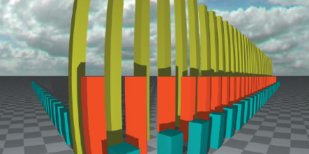
- 11.10. You can render square fisheye images by rendering all of the pixels. To do this, you just ignore the r2 < 1.0 inequality (11.2) in the render_scene and ray_direction functions. Figure 11.14(a) shows the scene in Figure 11.7(b) rendered in this manner, but you have to be careful with wide-angled views. If ψmax>180/√2, ψ will exceed 360° towards the corners of the square. You will also have to be careful with rectangular images. Figure 11.14(b) shows what will happen if you render the same scene with a pixel resolution of 600 × 300 pixels. Notice how everything is squashed in the vertical direction.
Figure 11.15 shows how Figure 11.14(b) should look. See if you can get the fisheye camera to render rectangular images without the distortion. Hint: one way to do this is to map the normalized device coordinates to a rectangle that has the same aspect ratio as the image and just fits into the disk in Figure 11.3(b).
- 11.11. Implement the Spherical camera and use Figures 11.11 and 11.12 for testing it. The boxes in this scene are randomly generated, and although I’ve seeded rand() in the build function, you may get different boxes, even with the same seed.
- 11.12. Render Figure 11.12 with the camera angled up or down and observe what happens to the vertical box edges.
- 11.13. Render spherical panoramic images with the horizontal fov > 360° and the vertical fov > 180°.
- 11.14. Implement a camera that renders cylindrical panoramic projections. This type of projection has a limited fov in the vertical direction but allows a 360° horizontal fov. In contrast to spherical panoramic projections, these have wide applications in immersive cylindrical viewing environments (see the Further Reading section).
1. This is a 4π steradian view in solid angle.
2. Normalized device coordinates can also be defined as (xn, y°) × [0, 1]2.
3. The clouds result from a spherical projection of an image onto a large sphere (radius 1000000), but it’s not a light source (see Chapter 29).