Chapter 21

Transforming Objects

Objectives

By the end of this chapter, you should:

• understand how to intersect rays with transformed objects;
• understand why instancing is the preferred method;
• be able to transform objects through instancing;
• understand how you can model numerous beveled objects.

In this chapter, I’ll put the theory of affine transformations into practice by explaining how to ray trace transformed objects. This will give you a lot of flexibility for modeling purposes.

21.1 Intersecting Transformed Objects

21.1.1 General Theory

How do we intersect rays with transformed objects? The answer is surprising and simple. We don’t! Suppose you wanted to ray trace an object with a specified set of affine transforms. Here are the steps:

• apply the inverse set of transformations to the ray to produce an inverse transformed ray;
• intersect the inverse transformed ray with the untransformed object;
• compute the normal to the untransformed object at the hit point;
• use the hit point on the untransformed object to compute where the original ray hits the transformed object;
• use the normal to the untransformed object to compute the normal to the transformed object.

Figure 21.1 illustrates these procedures, which are standard practice in ray tracing. They are also its neatest trick.

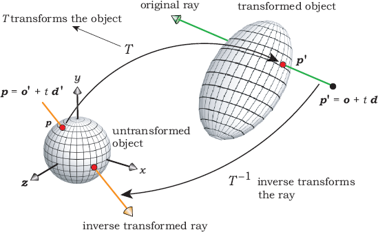
To carry out the above steps, consider a ray with origin o and direction d that hits the transformed object. We need to compute the coordinates of the nearest hit point p′ of this original ray and the transformed object. This point will satisfy

$p^{\prime }=o+t d,\text{ (21.1)}$

for some value of t.

There also exists a point p on the untransformed object that’s related to p′ by Equation (20.1):

$p^{\prime }=Tp,\text{ (21.2)}$

where T is the composite 4 × 4 transformation matrix of the form (20.10). If we multiply both sides of Equation (21.2) by the inverse transformation matrix T−1, we get

$p=T^{-1}{p}^{\prime }.\text{ (21.3)}$

To inverse transform the ray, we multiply both sides of Equation (21.1) by T−1, which gives

$T^{-1}{p}^{\prime }=T^{-1}o+t{T}^{-1}d.$

Using Equation (21.3), we can write this as

$p=o^{\prime }+t d^{\prime },\text{ (21.4)}$

where

$o^{\prime }=T^{-1}o\text{ (21.5)}$

and

$d^{\prime }=T^{-1}d\text{ (21.6)}$

are the inverse transformed ray origin and direction, respectively. Equation (21.4) is the inverse transformed ray. Figure 21.1 also illustrates this inverse transformation process.

21.1.2 Transforming Points and Vectors

We have to be careful with Equations (21.5) and (21.6) because o is a point and d is a vector, and as we saw in Chapter 20, these transform differently under affine transformations. As a reminder, points are affected by translation, but vectors are not affected.

Let’s write the inverse transformation matrix as

$T^{-1}=\left[\begin{array}{cccc}{m}_{00}& m_{01}& m_{02}& m_{03}\\ m_{10}& m_{11}& m_{12}& m_{13}\\ m_{20}& m_{21}& m_{22}& m_{23}\\ 0& 0& 0& 1\end{array}\right],$

where the rows and columns are numbered from zero instead of one.1 I’ll explain how to compute this matrix in Section 21.1.5.

To transform the ray origin, we represent it as a point in 4D homogeneous space o = [ox oy oz 1]T and multiply it on the left with T−1:

$o^{\prime }=\left[\begin{array}{cccc}{m}_{00}& m_{01}& m_{02}& m_{03}\\ m_{10}& m_{11}& m_{12}& m_{13}\\ m_{20}& m_{21}& m_{22}& m_{23}\\ 0& 0& 0& 1\end{array}\right]\left[\begin{array}{c}{o}_{\text{x}}\\ o_{\text{y}}\\ o_{\text{z}}\\ 1\end{array}\right].\text{ (21.7)}$

Writing out the first three components of Equation (21.7) gives

$\begin{array}{c}{o^{\prime }}_{\text{x}}=m_{00}{o}_{\text{x}}+m_{01}{o}_{\text{y}}+m_{02}{o}_{\text{z}}+m_{03},\\ {o^{\prime }}_{\text{y}}=m_{10}{o}_{\text{x}}+m_{11}{o}_{\text{y}}+m_{12}{o}_{\text{z}}+m_{13},\\ {o^{\prime }}_{\text{z}}=m_{20}{o}_{\text{x}}+m_{21}{o}_{\text{y}}+m_{22}{o}_{\text{z}}+m_{23}.\end{array}\text{ (21.8)}$

The transformation of the ray direction does not involve translation, a fact that’s handled very naturally in homogeneous coordinates, where directions can be represented by points with W = 0 (see the Further Reading section). Accordingly, we represent the ray direction as d = [dx dy dz 0]T so that

$d^{\prime }=\left[\begin{array}{cccc}{m}_{00}& m_{01}& m_{02}& m_{03}\\ m_{10}& m_{11}& m_{12}& m_{13}\\ m_{20}& m_{21}& m_{22}& m_{23}\\ 0& 0& 0& 1\end{array}\right]\left[\begin{array}{c}{d}_{\text{x}}\\ d_{\text{y}}\\ d_{\text{z}}\\ 0\end{array}\right].\text{ (21.9)}$

Writing out the components of Equation (21.9) gives

$\begin{array}{c}{d^{\prime }}_{\text{x}}=m_{00}{d}_{\text{x}}+m_{01}{d}_{\text{y}}+m_{02}{d}_{\text{z}},\\ {d^{\prime }}_{\text{y}}=m_{10}{d}_{\text{x}}+m_{11}{d}_{\text{y}}+m_{12}{d}_{\text{z}},\\ {d^{\prime }}_{\text{z}}=m_{20}{d}_{\text{x}}+m_{21}{d}_{\text{y}}+m_{22}{d}_{\text{z}}.\end{array}\text{ (21.10)}$

21.1.3 Programming Aspects

You will need a Matrix class that implements a 4 × 4 matrix. The Matrix class in the skeleton ray tracer stores the matrix elements in a public 4 × 4 C array called m. To transform 3D points according to Equations (21.8), I’ve overloaded the * operator in a non-member function defined in the file Point3D.cpp. This function appears in Listing 21.1. Note that the second parameter is a Point3D reference, not a 4D point; the code simply implements Equations (21.8).

Listing 21.2 shows the code for transforming a vector according to Equations (21.10).

Point3D

operator* (const Matrix& mat, const Point3D& p) {

      return (Point3D(mat.m[0][0] * p.x + mat.m[0][1] * p.y + mat.m[0][2] * p.z +

                         mat.m[0][3], 

                      mat.m[1][0] * p.x + mat.m[1][1] * p.y + mat.m[1][2] * p.z +

                         mat.m[1][3],

                      mat.m[2][0] * p.x + mat.m[2][1] * p.y + mat.m[2][2] * p.z +

                         mat.m[2][3]));

}

Listing 21.1. The function operator* that transforms a 3D point.

Vector3D 

operator* (const Matrix& mat, const Vector3D& v) {

     return (Point3D(mat.m[0][0] * v.x + mat.m[0][1] * v.y + mat.m[0][2] * v.z,

                mat.m[1][0] * v.x + mat.m[1][1] * v.y + mat.m[1][2] * v.z,

                mat.m[2][0] * v.x + mat.m[2][1] * v.y + mat.m[2][2] * v.z));

}

Listing 21.2. The function operator* that transforms a 3D vector. The function is in the file Vector3D.cpp.

21.1.4 Ray Intersection with Transformed Objects

The next step is to intersect the inverse transformed ray (21.4) with the untransformed object. Although this will often be a generic object, it could be any other type of object that’s being transformed, for example, a compound object. After we’ve found the closest hit point p on the untransformed object, we need to find the corresponding hit point p′ of the original ray with the transformed object. To do this, we use the following important property of the transformation process: if the closest hit point p of the inverse transformed ray with the untransformed object occurs at t = t0, the closest hit point p′ of the original ray with the transformed object occurs at the same value of t: t = t0.

The proof is as follows. From Equations (21.4)–(21.6),

$\begin{array}{cc}\hfill p& =o^{\prime }+t_0{d}^{\prime }\hfill \\ & =T^{-1}o+t_0{T}^{-1}d.\hfill \end{array}$

Multiplying both sides of this equation by T gives

$T_p=T{T}^{-1}o+t_0 T{T}^{-1}d=o+t_{0}d=p^{\prime },$

as required.

To find the hit point on the transformed object, we simply substitute t0 into the original ray Equation (21.1).

21.1.5 Inverse of the Transformation Matrix

From the above calculations, it’s clear that we need to compute the composite inverse transformation matrix for each transformed object. Fortunately, that’s not difficult because of the structure of the inverse matrix as given by Equation (20.14), which is reproduced here:

$T^{-1}=T_1^{-1}{T}_2^{-1}...T_{\text{n}}^{-1}.\text{ (21.11)}$

The inverse matrices for the individual transformations are all given in Section 20.5. You should compute the matrix (21.11) by multiplying the individual matrices on the right as each transformation is specified in a build function.

21.1.6 Example

The following is a simple example of a generic sphere that’s scaled, rotated, and translated. Figure 21.2 illustrates the transformations, starting with the generic sphere on the left and ending with the ellipsoid on the right. Specifically, the sphere is scaled by 2 in the x-direction and 3 in the y-direction, rotated −45° (clockwise) around the x-axis, and then translated 1 unit in the y-direction. Equation (21.12) shows the composite inverse transformation matrix that represents these transformations. Listing 21.7 demonstrates how these transformations can be specified in a build.

$T^{-1}=\underset{\text{inverse} \text{scale}}{\left[\begin{array}{cccc}1/2& 0& 0& 0\\ 0& 1/3& 0& 0\\ 0& 0& 1& 0\\ 0& 0& 0& 1\end{array}\right]}\underset{\text{inverse} \text{rotate}}{\left[\begin{array}{cccc}1& 0& 0& 0\\ 0& 1/\sqrt{2}& -1/\sqrt{2}& 0\\ 0& 1/\sqrt{2}& 1/\sqrt{2}& 0\\ 0& 0& 0& 1\end{array}\right]}\underset{\text{inverse} \text{translate}}{\left[\begin{array}{cccc}1& 0& 0& 0\\ 0& 1& 0& -1\\ 0& 0& 1& 0\\ 0& 0& 0& 1\end{array}\right]}.\text{ (21.12)}$

21.2 Transforming Normals

21.2.1 Theory

For shading purposes, we need the normal at the hit point on the transformed object. Fortunately, there’s a simple relationship between this normal and the normal at the hit point on the untransformed object. Although I’ll just quote the result here, you can find the derivation in Foley et al. (1995), p. 217, and Shirley et al. (2005), Chapter 6.

Let n be the normal to the untransformed object at the intersection with the inverse transformed ray, as illustrated in Figure 21.3. The normal n′ to the transformed object is given by

$n^{\prime }=T^{-T}{n}^{\prime },\text{ (21.13)}$

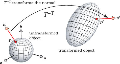
where T−T = (T−1)T is the transpose of the inverse transformation matrix. The normal transforms in this way because it has to remain perpendicular to the object surface (see Figure 2.8).

Do we have to store the transpose of T−1 in addition to T−1? No, because T−1 and T−T store the same information; the transpose of T−1 is simply obtained by swapping the rows and columns. Since normals are directions, we can represent these in homogeneous coordinates with W = 0, in the same way that we represent vectors. Normals are also not affected by translation. For a given inverse transformation matrix T−1 and normal n′ = [n′x n′y n′z 0] on the untransformed object, we can define the operation in Equation (21.13) by writing it in matrix form

$n={\left[\begin{array}{cccc}{m}_{00}& m_{01}& m_{02}& m_{03}\\ m_{10}& m_{11}& m_{12}& m_{13}\\ m_{20}& m_{21}& m_{22}& m_{23}\\ 0& 0& 0& 1\end{array}\right]}^{\text{T}}\left[\begin{array}{c}{n}_{\text{x}}\\ n_{\text{y}}\\ n_{\text{z}}\\ 0\end{array}\right]=\left[\begin{array}{cccc}{m}_{00}& m_{10}& m_{20}& 0\\ m_{01}& m_{11}& m_{21}& 0\\ m_{02}& m_{12}& m_{22}& 0\\ m_{03}& m_{13}& m_{23}& 1\end{array}\right]\left[\begin{array}{c}{n}_{\text{x}}\\ n_{\text{y}}\\ n_{\text{z}}\\ 0\end{array}\right].\text{ (21.14)}$

Normal

operator* (const Matrix& mat, const Normal& n) {

      return (Normal(    mat.m[0][0] * n.x + mat.m[1][0] * n.y + mat.m[2][0] * n.z,

                 mat.m[0][1] * n.x + mat.m[1][1] * n.y + mat.m[2][1] * n.z,

                 mat.m[0][2] * n.x + mat.m[1][2] * n.y + mat.m[2][2] * n.z));

}

Listing 21.3. The function operator* that transforms a normal. The function is in the file Normal.cpp.

Writing out the first three components of Equation (21.14) gives

$\begin{array}{c}{n^{\prime }}_x=m_{00}{n}_{\text{x}}+m_{10}{n}_{\text{y}}+m_{20}{n}_{\text{z}},\\ {n^{\prime }}_{\text{y}}=m_{01}{n}_{\text{x}}+m_{11}{n}_{\text{y}}+m_{21}{n}_{\text{z}},\\ {n^{\prime }}_{\text{z}}=m_{02}{n}_{\text{x}}+m_{12}{n}_{\text{y}}+m_{22}{n}_{\text{z}}.\end{array}\text{ (21.15)}$

21.2.2 Programming Aspects

The function that implements the transformation equations (21.15) appears in Listing 21.3. Because the resulting normal will not be of unit length, you will have to normalize it. Listing 21.6 illustrates where you should do this.

21.3 Directly Transforming Objects

There are two ways to implement transformations. One is directly in the objects, where we store the inverse transformation matrix in the GeometricObject class and provide a set of transformation functions to construct the matrix. We also have to store a Boolean variable that’s set to true when an object has been transformed.

This approach has a number of associated costs. The first is memory, as all objects then have to store the matrix whether they are transformed or not, and this requires 16 floats.2 This can significantly increase the memory footprint for large scenes, with an attendant increase in render times if it slows memory access.

The second cost is in the object hit functions. Listing 21.4 shows the plane hit function from Listing 3.5, amended to handle transformations. Here, we have to test if the object has been transformed and, if it has, compute the inverse transformed ray. This test is also required before the normal is computed. These tests take time.

bool

Plane::hit(const Ray& ray, double& tmin, ShadeRec& sr) const {

     if (transformed) {

          ray.o = inv_matrix * ray.o;

          ray.d = inv_matrix * ray.d;

     }

     float t = (a - ray.o) * normal  / (ray.d * normal );

     if (t > kEpsilon) {

          tmin = t;

          if (transformed) {

               sr.normal = inv_matrix * normal ;

               sr.normal.normalize();

          }

          else

               sr.normal = normal ;

          sr.local_hit_point = ray.o + t * ray.d;

          return (true); 

     }

     return (false);

}

Listing 21.4. Ray-plane hit function with affine transformations.

The third cost is programming effort because these tests and transformations have to be in the hit function and shadow_hit function of every object type.

21.4 Instancing

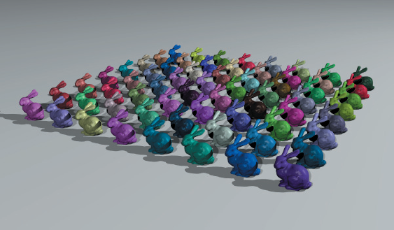
The second way to implement transformations is called instancing, and it avoids all of the above problems. To see what instancing is, consider an object that takes up a lot of memory, say a large triangle mesh with millions of triangles. Suppose we can only fit a few of these objects in memory, but we want to render a scene that contains a large number of them with different materials, locations, sizes, etc. We can do this by storing a single version of the object and constructing a number of instance objects that contain a pointer to the object, an inverse transformation matrix, and a material. We need a separate instance for each version of the object. Figure 21.4 shows an example where I’ve stored a single Stanford bunny but rendered it 64 times with different materials. I’ll explain after Listing 21.6 how each bunny was rendered with a different material.

The above example demonstrates how instances can save memory for large objects, but the memory savings are broader than that because we don’t have to store the matrix in the GeometricObject class. I’ve implemented instances in an Instance class that inherits from GeometricObject and can therefore have its own hit function where all of the transformation-specific code resides. This only has to be written once, and we don’t have to change the hit functions of any other objects to implement instancing.

Listing 21.5 shows part of the declaration for the class Instance. The transform_the_texture data member is used to attach textures to transformed objects, as I’ll explain in Chapter 29.

Listing 21.6 shows the Instance hit function. Although this is a short function, it performs a number of operations, some in subtle ways. You will need to study this function in conjunction with the functions World::hit_objects and Compound::hit because it can be called from these. In fact, this is the most connected function in the ray tracer. A couple of obvious facts are that it transforms a local copy of the ray, and it doesn’t test that the object is transformed. It can’t transform the ray parameter because that’s const, and for good reason. If any hit function changed the ray, the functions World::hit_objects and Compound::hit would not work; the same ray has to be tested against all objects. Something that may not be obvious is that operator * is overloaded in four ways. The first three are for transforming points, directions, and normals, as in Listing 21.1, Listing 21.2 and Listing 21.3, respectively, and the fourth is for multiplying a vector by a double on the left.

class Instance: public GeometricObject {

     public:

          Instance(void);

          Instance(const Object* obj_ptr);

          ...

          virtual bool

          shadow_hit(const Ray& ray, double& tmin) const;

          virtual bool

          hit(const Ray& ray, double& tmin, ShadeRec& sr) const;

          void

          translate(const float dx, const float dy, const float dz);

          // other transformation functions

     private:

          GeometricObject* object_ptr;     // object to be transformed

          Matrix inv_matrix;               // inverse transformation matrix

          bool transform_the_texture;      // do we transform the texture

};

Listing 21.5. Partial declaration of the class Instance.

bool

Instance::hit(const Ray& ray, float& t, ShadeRec& sr) const {

     Ray inv_ray(ray);

     inv_ray.o = inv_matrix * inv_ray.o;

     inv_ray.d = inv_matrix * inv_ray.d;

     if (object_ptr->hit(inv_ray, t, sr)) {

          sr.normal = inv_matrix * sr.normal;

          sr.normal.normalize();

          if (object_ptr->get_material())

               material_ptr = object_ptr->get_material();

          if (!transform_the_texture)

               sr.local_hit_point = ray.o + t * ray.d;

          return (true);

     }

     return (false);

}

Listing 21.6. The function Instance::hit.

What is not obvious is that the hit function is designed to work for arbitrarily nested instances, meaning that the stored object may be another instance. This is critical for modeling flexibility. When this happens, Instance::hit is called recursively until the object is untransformed.3 The ray is progressively inverse transformed before each recursive call so that the most transformed ray is ultimately intersected with an untransformed object.

Instance::hit also has to return the unit normal on the transformed object through its ShadeRec parameter. The object_ptr->hit function returns the unit normal n on the untransformed object, and the normal (21.13) on the transformed object is then progressively built up with the statement sr.normal = inv_matrix * sr.normal as the recursion stack unwinds. I’ve normalized the normal at each level because the code doesn’t keep track of the recursion depth and therefore has no way of knowing when it’s at the top level.

The code

if (object_ptr->get_material())

     material_ptr = object_ptr->get_material();

may look strange, but it performs a critical task. Each instance object has access to at least two materials. In the simplest case, the object being transformed will store a single material. This could be a primitive or something much more complex, such as one of the bunnies in Figure 21.4. The instance object also inherits a material pointer from GeometricObject, which has to be assigned a material somewhere before the hit function returns. If this isn’t done, the pointer will remain null, and the ray tracer could crash if it attempts to shade the transformed object. A simple guideline is as follows: If the build function assigns a material to the object being transformed, the instance hit function assigns this material to the instance material pointer. If the build function doesn’t assign a material to the object, it must assign a material to the instance. In this case, each instance of an object can have a different material (see Exercise 21.4).

The instance hit function checks if the object’s material pointer is not null before assigning it to its own material. It also correctly handles the case where the object being transformed is a compound object containing multiple materials. In this case, the Compound::hit function will return the correct material for the nearest primitive that the ray ultimately hits. A simple example is the multicolored ring in Figure 21.14, where each primitive component has its own material. A more complicated example is the bunnies in Figure 21.4, where the material for each triangle is not stored with the triangle but instead is stored in the grid.

In common with all hit functions, Instance::hit returns the minimum t value at the hit point when the ray hits the object. This is passed up the recursion stack without change.

I’ll discuss how the texture statement works in Chapter 30, because that’s most easily explained in a texturing context.

Listing 21.7 shows the build function for the ellipsoid on the right in Figure 21.2. Note the syntax used to construct the instance:

Instance* ellipsoid_ptr = new Instance(new Sphere);

This is the only statement that refers to the Instance class. The rendered result appears in Figure 21.5. Alternatively, you could construct a default instance object and set the object with an Instance::set_object function.

void

World::build(void) {

     vp.set_hres(400);

     vp.set_vres(400);

     vp.set_samples(16);

     tracer_ptr = new RayCast(this);

     Pinhole* camera_ptr = new Pinhole;

     camera_ptr->set_eye(100, 0, 100);

     camera_ptr->set_lookat(0, 1, 0);       

     camera_ptr->set_vpd(8000);

     camera_ptr->compute_uvw();

     set_camera(camera_ptr);

     PointLight* light_ptr = new PointLight();

     light_ptr->set_location(50, 50, 1);

     light_ptr->scale_radiance(3.0);

     add_light(light_ptr);

     Phong* phong_ptr = new Phong;

     phong_ptr->set_cd(0.75);

     phong_ptr->set_ka(0.25);

     phong_ptr->set_kd(0.8);

     phong_ptr->set_ks(0.15);

     phong_ptr->set_exp(50);

     Instance* ellipsoid_ptr = new Instance(new Sphere);

     ellipsoid_ptr->set_material(phong_ptr);

     ellipsoid_ptr->scale(2, 3, 1);

     ellipsoid_ptr->rotate_x(-45);

     ellipsoid_ptr->translate(0, 1, 0);

     add_object(ellipsoid_ptr);

}

Listing 21.7. The build function for the ellipsoid in Figure 21.2.

If an object constructor takes arguments, it can still be called with the instance constructor. For example:

Instance* box_ptr = new Instance (new Box(Point3D(-1, -1, -5), Point3D(1, 1, -3)));

As an example of the code that builds the inverse transformation matrix, Listing 21.8 shows the Instance::translate function. The other transformation functions are similar. The code in Listing 21.8 relies on the fact that the Matrix default constructor initializes a matrix to a unit matrix.

void

Instance::translate(const float dx, const float dy, const float dz) {

     Matrix inv_translation_matrix;     // temporary matrix

     inv_translation_matrix.m[0][3] = -dx;

     inv_translation_matrix.m[1][3] = -dy;

     inv_translation_matrix.m[2][3] = -dz;

     // post-multiply for inverse translation

     inv_matrix = inv_matrix * inv_translation_matrix;

}

Listing 21.8. The function Instance::translate.

To summarize: The benefits of using instances to transform objects are that object hit functions are simpler and run marginally faster and the transformation code only has to be written once. Objects are also smaller because the matrix is only stored in the instances. The disadvantages are that the transformed object hit functions are accessed through an additional indirection and the build-function syntax is slightly more complex.

At this stage, the Instance class is not complete, as we still have to deal with the issue of computing and storing the (forward) transformation matrix. I’ll cover that in Chapter 22. The Instance::hit function is, however, in its final form.

21.5 Beveled Objects

Figure 21.6 shows three compound objects that we can model using the objects from Chapter 19 and transformations. Here, each object has been transformed.

Figure 21.7 shows beveled versions of these objects, where the sharp edges are now rounded. This is a more accurate way of modeling many common objects, which often have rounded edges. The beveling also creates more interesting images because the bevels can show specular highlights.

Beveling is common in commercial modeling and rendering packages, where it’s usually implemented using triangle meshes. In contrast, we have enough primitives at our disposal to model a number of parameterized beveled objects, such as those shown in Figure 21.7, without using triangles. Why discuss beveling here, and not in Chapter 19? The reason is that the untransformed versions of these beveled objects all contain transformed components.

The beveled cylinder is particularly simple to model, as the exploded view in Figure 21.8(a) indicates. We just add two tori to the solid cylinder from Chapter 19 and parameterize it with the minimum and maximum y values, the cylinder radius, and the bevel radius. Figure 21.8(b) shows how the parts fit together. Note that only a quarter of each torus is visible. The catch is that the tori have to be translated in the y direction.

Listing 21.9 shows a constructor for the BeveledCylinder class that illustrates how to construct the bevels. You should compare this with Listing 19.14 for the solid cylinder.

The beveled box is by far the most complex object in Figure 21.7, with 26 components: eight spheres, six rectangles, and 12 open cylinders. The use of a bounding box considerably speeds the rendering of this object. See Listing 19.15 for an example of how to do this.

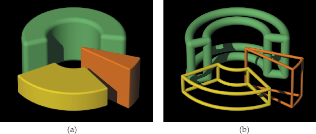
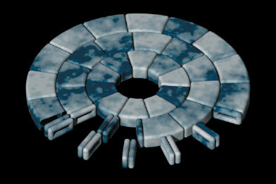
Finally, Figure 21.9(a) shows three examples of a beveled wedge object. This is the most complex beveled object in the collection, with 30 primitives: eight spheres, eight open cylinders, two part cylinders, four part tori, two rectangles, and six part annuli. Figure 21.9(b) shows the same objects as in Figure 21.9(a) with part of their outer surfaces removed.

BeveledCylinder::BeveledCylinder(const float  bottom,

         const float     top,

         const float     radius,

         const float     bevel_radius)

         : Compound() {

      objects.push_back(new Disk(Point3D(0, bottom, 0),               // bottom

                 Normal(0, -1, 0), 

                 radius - bevel_radius));  

      objects.push_back(new Disk(Point3D(0, top, 0),                  // top

                 Normal(0, 1, 0), 

                 radius - bevel_radius));   

      objects.push_back(new OpenCylinder(bottom + bevel_radius,       // vertical wall

                 top - bevel_radius, 

                 radius));  

      Instance* bottom_bevel_ptr = new Instance(new Torus(radius - bevel_radius,

                                                bevel_radius));

      bottom_bevel_ptr->translate(0, bottom + bevel_radius, 0);

      objects.push_back(bottom_bevel_ptr);

      Instance* top_bevel_ptr = new Instance(new Torus(radius - bevel_radius,

                                             bevel_radius));

      top_bevel_ptr->translate(0, top - bevel_radius, 0);

      objects.push_back(top_bevel_ptr);

}

Listing 21.9. A parameterized constructor for the BeveledCylinder class.

Figure 21.10 shows a top-down view of a beveled wedge. The parameters are the y extents y0, y1, the inner and outer radii r0, r1, the minimum and maximum azimuth angles φ0, φ1, and the bevel radius br. The bevel radius is the common radius of the spheres, open cylinders, and part tori. The beveled wedge class is on the book’s website.

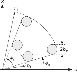
There are a number of restrictions on the parameters: we must have r1 > r0 > 0 with minimum separations between 0, r0, and r1 that depend on the other parameters, particularly br; similarly, we must have y1 > y0 and 0° < φ0 < φ1 < 360° with minimum separations. Setting φ0 = 0° and φ1 = 360° will not result in a beveled thick ring like the one illustrated in Figure 21.7 (see Figure 21.17).

In spite of these limitations, the beveled wedge is a most useful modeling object, particularly for architecture. Figure 21.11 shows two examples using noise-based textures from Chapter 31. Figure 21.11(a) is a rosette rendered with marble; Figure 21.11(b) is a wall with an archway rendered with marble and sandstone. The beveled wedges in these figures were stored in grids to improve the rendering times. Because of their complexity, a tight bounding box is critical for reasonable rendering times, particularly when large numbers of the wedges are stored in a grid. A trivial bounding box is p0 = (−r1, y0, −r1), p1 = (r1, y1, r1), and it’s also possible to compute a reasonably tight bounding box when r1 − r0 << r1 and φ1 − φ0 << 360°. The complete BeveledWedge class is on the book’s website.

Further Reading

Hill (1990) was the first general graphics textbook to discuss transformations in ray tracing but used 3 × 3 matrices to represent scaling, rotation, reflection, and shearing and a vector to represent translation. The most recent edition of Hill and Kelley (2006) uses 4 × 4 matrices. Wilt (1994) has transformations in the code as 4 × 4 matrices but doesn’t appear to discuss them in the text. Shirley and Morley (2003) discusses transformations the way I’ve implemented them using instancing. The main difference between the two implementations is that they use a single class for vectors, points, and normals. The first edition of this book, Shirley (2000), was the inspiration for my use of instances.

Notes and Discussion

The Instance Hit Function

I wish I could say that I wrote the Instance::hit function in one go, but I didn’t. This function evolved over several years as I added features to the ray tracer that it couldn’t handle. The part that gave me the most trouble was the if statement for transforming the texture. I’ll discuss this in Chapter 30.

Transformation Code

You will need to perform transformations on textures as well as geometric objects, and you may also want to transform the camera. With the current architecture, you will end up with repeated transformation code. A possible way to avoid this is to provide a transforms class whose objects can provide transformation services to other objects. This could encapsulate all of the transformations code in one place, but before you try this, you need to read Chapter 22. As it turns out, not all objects require the same transformation code. Instances need extra code in their transformation functions so that we can place transformed objects in grids. Textures and bump maps don’t need this extra code. There’s also the issue of transforming area lights with their sample points (see Exercise 21.15).

Important Point

Transforming the direction with Equations (21.10) can result in a ray direction that is not a unit vector when the inverse transformed ray is intersected with the object in the function Instance::hit. This is why you should not assume that the ray direction is a unit vector in any hit function.

Questions

• 21.1.  Which transformations can change the length of the ray direction?
• 21.2.  Which transformations can change the length of the normal?
• 21.3.  The last statement in Listing 21.8 is inv_matrix = inv_matrix * inv_translation_matrix;. Suppose this were the first transformation that you applied to an object. What should the matrix inv_matrix be on the right-hand side of the assignment? How can you make sure it will always be this matrix in this situation? Is this question relevant to the other transformations?
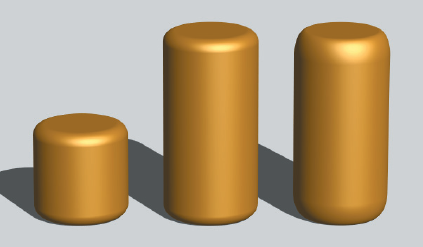
• 21.4.  The middle beveled cylinder in Figure 21.12 was constructed to be twice the height of the left cylinder. The right cylinder was constructed to be the same height as the left cylinder and was then scaled by a factor of two in the y-direction. Why is this different from the middle cylinder? The bevel radius is the same for all cylinders.

  Figure 21.12

  

  Three beveled cylinders.

• 21.5.  Figure 21.13 shows a nice speckled sphere with holes, except that it’s not really a sphere. It’s a beveled cylinder with y0 = −1, y1 = 1, radius = 1, and bevel radius = 1. Can you explain what has happened?

  Figure 21.13

  

  A speckled sphere. Notice the shadow visible through the sphere and the speckles of light in the shadow.

Exercises

• 21.1.  Implement instances and test your code with the ellipsoid in Figure 21.5.
• 21.2.  Figure 21.14 shows a multicolored thick ring that has been rotated and translated, using a nested instance object. See the build-function code fragment in Listing 21.10. Use this as a further test of your Instance class. The complete build function is on the book’s website.

  Instance* rotated_ring_ptr = new Instance(ring_ptr);

  rotated_ring_ptr->rotate_z(-45);

  Instance* translated_ring_ptr = new Instance(rotated_ring_ptr);

  translated_ring_ptr->translate(1, 0, 0);

  add_object(translated_ring_ptr);

  Listing 21.10. Code fragment from the build function for Figure 21.14.

  Figure 21.14

  

  Transformed multicolored ring with shadows.

• 21.3.  Write the function Instance::shadow_hit and test that shadows work correctly with instances. You can use Figure 21.14 for testing purposes because the ring: casts a shadow on the plane, self-shadows, and has a shadow cast on it by the sphere.
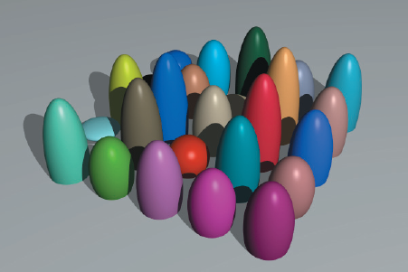
• 21.4.  Figure 21.15 shows 25 randomly colored ellipsoids constructed from a single generic sphere. Use this image to test the ability of the Instance class to create multiple transformed objects with different materials. Although I have seeded rand to generate these ellipsoids, you may get different colors and shapes.

  Figure 21.15

  

  Ellipsoids generated from a single generic sphere, which is not rendered.

• 21.5.  Apply further transformations to the ellipsoid in Figure 21.5 but, as always, be careful with their order.
• 21.6.  Figures 19.27(b) and 19.28(b) show a generic hemispherical bowl with a rounded rim. If you have implemented this, the simplest way to render this type of bowl in arbitrary locations, etc., is to use instances to transform it. Experiment with this.

• 21.7.  Figure 21.16(a) shows the definition of a slightly more general round-rimmed bowl that has an arbitrary opening angle at the top. It consists of a translated torus for the rim and two part spheres centered on the origin. The simplest way to specify the opening angle is to use θmin, as indicated in Figure 21.16(a), because then θmin is also the minimum polar angle for the part spheres, as illustrated in Figure 19.18(a). The actual opening angle will be smaller than this because half of the torus is inside the cone defined by the y-axis and θmin, but that’s not as easy to work with.

  Figure 21.16

  

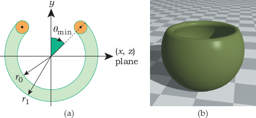
  (a) Definition of a round-rimmed bowl; (b) rendered bowl with an opening angle of 120°.

  To model the rim, we start with a generic torus with parameters

  $\begin{array}{c}a=\left[\left(r_1+r_2\right)/2\right]sin{\theta }_{min},\\ b=\left(r_2-r_1\right)/2\end{array}$

  and translate it by [(r1 + r2)/2] cos θmin in the y-direction.

  Part of the rim and the outer part sphere will be components of a spherical fishbowl, to be discussed in Chapter 28. Implement this bowl and use Figure 21.16(b) to test it. Note the apparent anomalous specular highlight shading when the highlight on the sphere hits the torus. This is correct, but try to work out why it happens. Here are some hints. The curvature of the torus is quite different from the curvature of the sphere, and the specular highlights are a different shape. You can see this from the specular highlight on the back of the rim. Render the bowl without the outer sphere. Also, render the bowl with its center, the eye point, and the (point) light location in a straight line and note how the anomalous shading disappears.

• 21.8.  Implement the objects in Figure 21.6 and render this scene.

• 21.9.  Implement the beveled objects in Figure 21.7 and render this scene. Experiment with different parameters, for example, the bevel radii.

  Implement bounding boxes for these beveled objects and compare the rendering speeds.

• 21.10.  Get the beveled wedge object running in your ray tracer and test it with Figure 21.9(a).
• 21.11.  Reproduce the rosette and archway images in Figure 21.11.
• 21.12.  If you look closely at the rosette in Figure 21.11(a), you’ll notice that the radial edges of several wedges line up. The reasons are as follows. Three edges line up on the left because the first wedge in each ring starts with φ0 = 0. Other edges line up because the number of wedges in each ring must divide 360 a whole number of times, and there’s not a huge choice of numbers to pick from. From the inner to the outer ring, I’ve used 10, 12, and 15 wedges. You may think that a simple way to prevent this alignment would be to add an offset to φ0 in each ring, which rotates the wedges around the y-axis, but this will not work. Figure 21.17 shows the results of using offsets of zero for the inner ring, 63° for the middle ring, and 126° for the outer ring. What has happened here? Why are some parts of the wedges rendered and not others? Can you think of a solution?

  Figure 21.17

  

  The result of adding offsets to the φ0 angles in the outer two rings.

• 21.13.  Put mortar between the wedges and blocks in the rosette, the archway, and the wall in Figure 21.11.
• 21.14.  Use beveled wedges and beveled boxes to produce some nice images of your own. A medieval castle would look good.
• 21.15.  Implement a technique that will allow you to transform area lights. The instance mechanism described here will allow you to transform the area light objects but not the sample points on them.

1. This makes the notation in the following equations correspond more closely to the code if you use a 2D array in C to store the matrix elements.

2. You could get by with 12 floats if you don’t store the last row.

3. An untransformed compound object could still have transformed components, as the beveled cylinder discussed in Section 21.5 demonstrates. Any transformed components would trigger further recursive calls.